线性代数 · SVD | 奇异值分解命名来历与直观理解

注：本文为 “线性代数 · SVD” 相关讨论合辑。
英文引文，机翻未校。
图片清晰度受引文原图所限。
略作重排，如有内容异常，请看原文。

---

Why is the SVD named so?

为什么奇异值分解（ SVD ）会如此命名？

The SVD stands for Singular Value Decomposition. After decomposing a data matrix $X$ using SVD , it results in three matrices, two matrices with the singular vectors $U$ and $V$, and one singular value matrix whose diagonal elements are the singular values. But I want to know why those values are named as singular values. Is there any connection between a singular matrix and these singular values?
奇异值分解（ SVD ）全称为 Singular Value Decomposition。使用 SVD 对数据矩阵 $X$ 进行分解后，会得到三个矩阵：两个分别由奇异向量构成的矩阵 $U$ 和 $V$，以及一个奇异值矩阵（其对角元素为奇异值）。但我想知道，这些值为何被命名为“奇异值”？奇异矩阵与这些奇异值之间是否存在关联？

edited May 30, 2023 at 6:14
Rodrigo de Azevedo
asked Apr 13, 2013 at 8:42
S. P

• wikipedia / Singular_value_decomposition #History
  维基百科：奇异值分解 # 历史

  – Jean-Claude Arbaut
  Commented Apr 13, 2013 at 8:43

• Hi @arbautjc, my question was not about history of singular values. Why those values are called as singular values. Is there any proper scientific reason? or are they connected with singular matrix (non-invertible).
  嗨 @arbautjc，我的问题并非关于奇异值的历史。我想知道这些值为何被称为“奇异值”，是否存在合理的科学依据？或者它们与奇异矩阵（不可逆矩阵）之间有关联？

  – S. P
  Commented Apr 13, 2013 at 10:12

• 1

  “Is there any connection between singular matrix and these singular values?” - in name, no. But it is true that if the matrix has singular values equal to zero, then the matrix is singular.
  “奇异矩阵与这些奇异值之间是否存在关联？”——从名称来源上看，没有关联。但一个事实是：若矩阵存在等于 0 的奇异值，则该矩阵为奇异矩阵。

  – J. M. ain’t a mathematician
  Commented Apr 13, 2013 at 12:53

• 1

  @S.P I know, but it’s to be found in history of mathematics.
  @S.P 我明白你的意思，但这个问题的答案需要从数学史中寻找。

  – Jean-Claude Arbaut
  Commented Apr 13, 2013 at 18:14

• 2

  “One of the miseries of life is that everybody names things a little bit wrong, and so it makes everything a little harder to understand.” _ – Feynman
  “生活的烦恼之一在于，人们给事物命名时总有些偏差，这使得一切都变得更难理解。”——费曼

  – littleO
  Commented May 30, 2023 at 0:34

3 Answers

From On the Early History of the Singular Value Decomposition_ by Pete Stewart:
引自皮特·斯图尔特（Pete Stewart）的论文《奇异值分解的早期历史》：

The term “singular value” seems to have come from the literature on integral equations. A little after the appearance of Schmidt’s paper, Bateman refers to numbers that are essentially the reciprocals of the eigenvalues of the kernel as singular values. Picard combined Schmidt’s results with Riesz’s theorem on the strong convergence of generalized Fourier series to establish a necessary and sufficient condition for the existence of solutions of integral equations.
“奇异值”（singular value）这一术语似乎源自积分方程相关文献。在施密特（Schmidt）的论文发表后不久，贝特曼（Bateman）将一种本质上为“核（kernel）的特征值的倒数”的数值称为“奇异值”。皮卡德（Picard）将施密特的研究结果与里斯（Riesz）关于“广义傅里叶级数强收敛性”的定理相结合，确立了积分方程解存在的充要条件。
 
In a later paper on the same subject, he notes that for symmetric kernels Schmidt’s eigenvalues are real and in this case (but not in general) he calls them singular values. By 1937, Smithies was referring to singular values of an integral equation in our modern sense of the word. Even at this point, usage had not stabilized. In 1949, Weyl speaks of the “two kinds of eigenvalues of a linear transformation,” and in a 1969 translation of a 1965 Russian treatise on nonselfadjoint operators Gohberg and Krein refer to the “s-numbers” of an operator.
在后续一篇关于同一主题的论文中，皮卡德指出：对于对称核，施密特定义的特征值为实数，且在这种情况下（而非普遍情况），他将这些特征值称为“奇异值”。到 1937 年，史密斯（Smithies）所指的“积分方程的奇异值”已与我们如今对该术语的理解一致。即便在此时，“奇异值”的用法仍未完全固定：1949 年，外尔（Weyl）将其表述为“线性变换的两种特征值”；而在 1969 年翻译的、1965 年出版的一本关于“非自伴算子”的俄语专著中，戈德堡（Gohberg）与克雷恩（Krein）则将其称为算子的“s-数”（s-numbers）。

See the paper for more fascinating accounts on how SVD came to be, even before the seminal paper of Golub/Kahan.
若想了解更多关于奇异值分解（ SVD ）发展历程的有趣内容（甚至包括戈卢布/卡汉（Golub/Kahan）的开创性论文发表之前的相关历史），可参考上述论文。

edited Jun 12, 2020 at 10:38
answered Apr 13, 2013 at 12:50
J. M. ain’t a mathematician

• I have long forgotten the term “s-number”. Your answer makes me feel nostalgic!
  我早就忘了“s-数”这个术语了，你的回答让我很有怀旧感！

  – user1551
  Commented Apr 13, 2013 at 13:53

• Why, thank you. Reading Pete Stewart’s paper made me feel fuzzy, too. On the other hand, nowadays I’m doing way more linear algebra and way less operator theory…
  哎呀，谢谢你的认可。读皮特·斯图尔特的论文也让我颇有感触。不过现在我研究线性代数的时间要多得多，算子理论则接触得少了……

  – J. M. ain’t a mathematician
  Commented Apr 13, 2013 at 14:05

2

From Schwartzman’s The Words of Mathematics_:
引自施瓦茨曼（Schwartzman）所著《数学术语》：

singular (adjective), singularity (noun): from Latin singulus “separate, individual, single,” from the Indo-European root sem- “one, as one.” If there is just a single example of something, that example becomes special, so singular took on the meaning “out of the ordinary.” […] The meaning “out of the ordinary, troublesome,” explains why a singular matrix is a square matrix whose determinant equals 0 rather than 1, as the etymology implies.
singular（形容词，译为“奇异的”）、singularity（名词，译为“奇点”）：源自拉丁语 singulus，意为“分离的、个别的、单一的”，其词根可追溯至印欧语系的 sem-（表示“一、作为一个整体”）。若某事物仅有唯一实例，该实例便会显得特殊，因此 singular 逐渐衍生出“非同寻常的”这一含义……正是“非同寻常的、有问题的”这一含义，解释了为何“奇异矩阵”（singular matrix）指的是行列式为 0（而非 1）的方阵——这与词源所暗示的含义一致。

Also, note that the terms singular matrix and singular value are contemporary. They made their first documented appearance in 1907 and 1908, respectively.
此外需注意，“奇异矩阵”（singular matrix）与“奇异值”（singular value）这两个术语属于同一时期的产物，其首份有记载的出现时间分别为 1907 年和 1908 年。

As such, I’d guess that singular values are called like that just because they are indeed out of the ordinary. They provide a nice invariant for any complex valued matrix.
因此，我推测“奇异值”之所以被如此命名，仅仅是因为它们确实具有“非同寻常”的性质——它们为任意复值矩阵提供了一种优良的不变量。

edited Jul 30, 2016 at 4:41
J. M. ain’t a mathematician
answered Apr 13, 2013 at 11:36
A.P.

“Singular” means “noninvertible,” and any eigenvalue $\lambda$ of matrix $M$ makes $M-\lambda I$ a singular (that is, noninvertible) matrix.
“Singular”（奇异的）意为“不可逆的”：对于矩阵 $M$ 的任意特征值 $\lambda$，矩阵 $M-\lambda I$ 均为奇异矩阵（即不可逆矩阵）。

The singular values $\sigma$ of $A$ are the values for which the matrices
矩阵 $A$ 的奇异值 $\sigma$ 是满足以下条件的数值：矩阵

$A^{\top }A-{\sigma }^{2}I$
$A{A}^{\top }-{\sigma }^{2}I$

are singular (noninvertible).
均为奇异矩阵（即不可逆矩阵）。

See https://en.wikipedia.org/wiki/Singular_value#History :
参考链接：（维基百科：奇异值#历史）：

This concept [of singular values] was introduced by Erhard Schmidt in 1907. Schmidt called singular values “eigenvalues” at that time. The name “singular value” was first quoted by Smithies in 1937.
“奇异值”这一概念由埃哈德·施密特（Erhard Schmidt）于 1907 年提出，当时施密特将其称为“特征值”（eigenvalues）。而“奇异值”（singular value）这一名称则由史密斯（Smithies）于 1937 年首次引用。

Additionally (and this may simply be fortuitous coincidence), the singular vectors of $A$ are two sets of vectors, {vi}\{ v_i \}{vi​} and {ui}\{ u_i \}{ui​}, such that for any $v_i$, then $A{v}_i={\sigma }_i{u}_i$. The image of each singular vector $v$ is therefore a multiple of a single singular vector $u$! Thus, singular vectors are vectors that map to multiples of single singular vectors.
此外（这可能只是偶然的巧合），矩阵 $A$ 的奇异向量分为两组，即 {vi}\{ v_i \}{vi​}（右奇异向量）和 {ui}\{ u_i \}{ui​}（左奇异向量），且满足：对任意 $v_i$，均有 $A{v}_i={\sigma }_i{u}_i$。也就是说，每个奇异向量 $v$ 在矩阵 $A$ 作用下的像（image），是某个“单一”（single）奇异向量 $u$ 的倍数！因此，“奇异向量”（singular vectors）指的是“映射后为单一奇异向量倍数”的向量——这也从侧面呼应了“singular”（与“single”同源）的词源含义。

edited Jun 2, 2023 at 16:39
answered May 30, 2023 at 0:21
SRobertJames

---

Understanding the singular value decomposition ( SVD )

理解奇异值分解（ SVD ）

Please, would someone be so kind and explain what exactly happens when Singular Value Decomposition is applied on a matrix? What are singular values, left singular, and right singular vectors? I know they are matrices of specific form, I know how to calculate it but I cannot understand their meaning.
请问有人能好心解释一下：对矩阵应用奇异值分解（ SVD ）时，具体会发生什么？什么是奇异值、左奇异向量和右奇异向量？我知道它们是特定形式的矩阵，也知道如何计算，但无法理解其含义。

I have recently been sort of catching up with Linear Algebra and matrix operations. I came across some techniques of matrix decomposition, particularly Singular Value Decomposition and I must admit I am having problem to understand the meaning of SVD .
最近我在补线性代数和矩阵运算的相关知识，接触到了一些矩阵分解技术，其中尤其对奇异值分解（ SVD ）感到困惑——我实在难以理解它的核心含义。

I read a bit about eigenvalues and eigenvectors only because I was interested in PCA and I came across diagonalizing a covariance matrix which determines its eigenvectors and eigenvalues (to be variances) towards those eigenvectors. I finally understood it but SVD gives me really hard time.
我之前为了了解主成分分析（PCA），读了一些关于特征值和特征向量的内容：对协方差矩阵进行对角化后，得到的特征向量对应“主成分方向”，特征值则对应这些方向上的方差——这个过程我终于理解了，但奇异值分解（ SVD ）还是让我感到棘手。

thanks

edited Aug 19, 2020 at 16:00
Rodrigo de Azevedo
asked Jun 4, 2013 at 22:46
Celdor

• 7
  The rough idea is that whereas a matrix $A$ can fail to be diagonalizable, the matrix $A^{\ast }A$ is always a nice semidefinite positive hermitian matrix, whence diagonalizable in an orthonormal basis with nonnegative eigenvalues. The singular values of $A$ are just the square roots of the latter. A SVD decomposition exploits that. There is more to say, but that’s a start.
  大致思路是这样的：虽然矩阵 $A$ 可能无法对角化，但矩阵 $A^{\ast }A$（$A^{\ast }$ 表示共轭转置）始终是一个性质良好的半正定埃尔米特矩阵（positive semidefinite Hermitian matrix），因此它能在标准正交基下对角化，且所有特征值均为非负数。而矩阵 $A$ 的奇异值，正是这些特征值的平方根。奇异值分解（ SVD ）的核心思想就源于这一特性。相关内容还有很多，但这可以作为理解的起点。

  – Julien
  Commented Jun 4, 2013 at 22:55

• Thanks @julien. Thanks for your comment. I read what are singular values in the $D$ matrix. I know they are square roots of eigenvalues of $A^{T}A$. What I don’t understand is the meaning? I know if I e.g. take covariance matrix and diagonalize it, I end up with eigenvalues (or maximum/unique/?singular? values) in a diagonal matrix representing variances. ** SVD ** however is product of three matrices: outer product o, singular values, inner product of A. But I still don’t see the meaning of all this.

  谢谢 @julien，感谢你的评论。我了解到奇异值是矩阵 $D$（奇异值矩阵）中的元素，也知道它们是 $A^{T}A$（$A$ 的转置与自身的乘积）特征值的平方根。但我不理解的是“含义”——比如，我知道对协方差矩阵对角化后，对角矩阵中的特征值代表“方差”，这一点很明确。可奇异值分解（ SVD ）是三个矩阵的乘积：（我理解的）外积、奇异值、矩阵 $A$ 的内积，但我还是看不出这一切背后的意义。

  – Celdor
  Commented Jun 5, 2013 at 2:55

• A related problem.
  这是一个相关问题（可参考其他讨论）。

  – Mhenni Benghorbal
  Commented Aug 26, 2013 at 22:45

• See stats.stackexchange.com/questions/177102
  可参考统计学领域关于 SVD 的相关讨论

  – kjetil b halvorsen
  Commented Nov 3, 2015 at 19:58

• 1

  I wrote an explanation of the SVD here: stats.stackexchange.com/a/403924/43159 If $A$ is a real $m\times n$ matrix, it’s natural to ask in which direction $v$ does $A$ have the most amplifying power. So, we define $v_1$ to be the unit vector $v$ that maximizes $\Vert Av\Vert$. This direction $v_1$ is the most important direction for understanding $A$. The next most important direction $v_2$ is the unit vector that maximizes $\Vert Av\Vert$ subject to the constraint that $v$ is orthogonal to $v_1$. Continuing like this, this thought process leads directly to the SVD of $A$.
  我在这个链接中写过关于 SVD 的解释：stats.stackexchange.com/a/403924/43159。简单来说：若 $A$ 是一个实 $m\times n$ 矩阵，一个很自然的问题是“矩阵 $A$ 在哪个方向 $v$ 上的‘放大能力’最强？”。因此，我们定义 $v_1$ 为“使 $\Vert Av\Vert$（向量 $Av$ 的模长）最大的单位向量”，这个方向 $v_1$ 是理解矩阵 $A$ 作用的“最重要方向”。接下来，第二重要的方向 $v_2$ 是“在与 $v_1$ 正交的前提下，使 $\Vert Av\Vert$ 最大的单位向量”。以此类推，这个思考过程会直接导出矩阵 $A$ 的奇异值分解（ SVD ）。

  – littleO
  Commented Jan 12, 2021 at 10:48

7 Answers

One geometric interpretation of the singular values of a matrix is the following. Suppose $A$ is an $m\times n$ matrix (real valued, for simplicity). Think of it as a linear transformation ${\mathbb{R}}^n\to {\mathbb{R}}^m$ in the usual way. Now take the unit sphere $S$ in ${\mathbb{R}}^n$. Being a linear transformation, $A$ maps $S$ to an ellipsoid in ${\mathbb{R}}^m$. The lengths of the semi-axes of this ellipsoid are precisely the non-zero singular values of $A$. The zero singular values tell us what the dimension of the ellipsoid is going to be: $n$ minus the number of zero singular values.
矩阵奇异值的一种几何解释如下：假设 $A$ 是一个 $m\times n$ 实矩阵（为简化理解，此处限定为实矩阵），我们将其视为从 ${\mathbb{R}}^n$（n维欧几里得空间）到 ${\mathbb{R}}^m$（m维欧几里得空间）的线性变换。取 ${\mathbb{R}}^n$ 中的单位球面 $S$（所有模长为1的n维向量构成的集合），由于 $A$ 是线性变换，它会将单位球面 $S$ 映射为 ${\mathbb{R}}^m$ 中的一个椭球面。这个椭球面的“半长轴长度”，恰好就是矩阵 $A$ 的非零奇异值；而零奇异值的数量则决定了椭球面的维度——具体为 $n$（原空间维度）减去零奇异值的个数。

answered Aug 26, 2013 at 22:20
Ittay Weiss

• Hi Ittay Wiess. I followed your explanation. Thanks. I can guess that if $S$ already has different diagonal values than 1 meaning $S$ is different from $I$, then it will already be sort of n-dim ellipsoid. To this whole picture, I would need to know what the other matrices are responsible for? Can you give me similar geometric explanation for them? I will be grateful. I am guessing is it just that one of them rotates and the other skew this sphere/ellipsoid ellipsoid.
  嗨，伊泰·维斯（Ittay Weiss）。我理解了你的解释，谢谢！我能猜到：如果单位球面 $S$ 对应的矩阵（比如缩放矩阵）对角元素不等于1（即该矩阵不等于单位矩阵 $I$），那么它本身就会是一个n维椭球面。但对于 SVD 的完整图景，我还想知道另外两个矩阵（左奇异向量矩阵 $U$ 和右奇异向量矩阵 $V$）分别起什么作用？你能给我一个类似的几何解释吗？非常感谢！我猜是不是其中一个矩阵负责“旋转”，另一个负责“扭曲”这个球面/椭球面？

  – Celdor
  Commented Sep 27, 2013 at 13:57

22

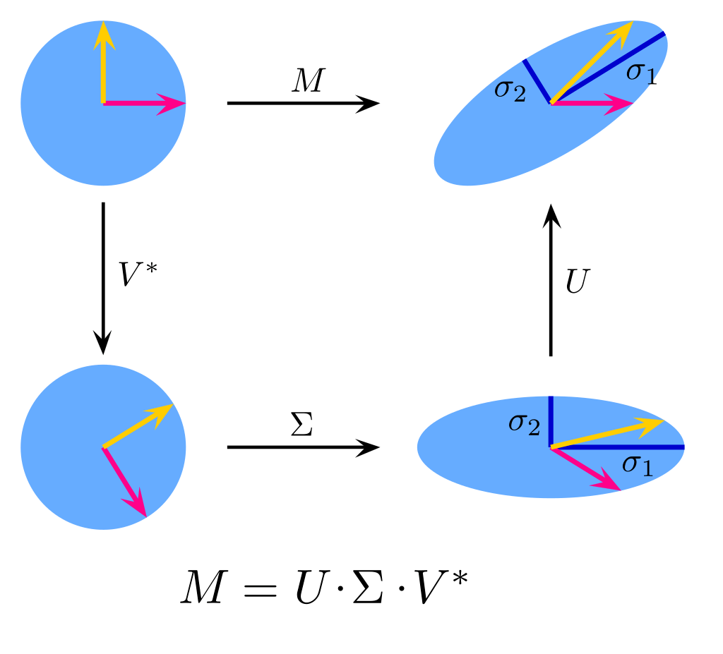
Think of a matrix $A$ as a transformation of space. SVD is a way to decompose this transformation into a series of three consecutive, canonical transformations: a first rotation, scaling and a second rotation. There is a nice picture on Wikipedia showing this transformation:
我们可以将矩阵 $A$ 理解为“空间的一种变换”，而奇异值分解（ SVD ）则是将这种变换“拆解”为三个连续的、标准的基本变换：第一次旋转、缩放、第二次旋转。维基百科上有一张很好的图展示了这个过程，图中清晰呈现了“旋转→缩放→旋转”的步骤。

Another thing that helps to build the intuition is to derive the equation yourself. For any matrix $A$ of size $n\times m$ the row space and a column space will be subspaces of ${\mathbb{R}}^m$ and ${\mathbb{R}}^n$ respectively. You are looking now for a orthonormal basis of a row space of $A$, say $V$, that gets transformed into the column space of $A$ such that it remains an orthonormal basis (in the column space of $A$). Let’s call this transformed basis $U$. So each $v_i$ get’s mapped to some $u_i$, possibly with some stretching, say scaled by ${\sigma }_i$:
另一个帮助建立直觉的方法是亲自推导 SVD 的核心方程。对于任意 $n\times m$ 矩阵 $A$，其行空间（row space）是 ${\mathbb{R}}^m$ 的子空间，列空间（column space）是 ${\mathbb{R}}^n$ 的子空间。我们需要找到行空间的一组标准正交基 $V$（即右奇异向量构成的基），使得这组基在经过矩阵 $A$ 变换后，能成为列空间的一组标准正交基 $U$（即左奇异向量构成的基）——不过变换过程中可能会有“拉伸”，即每个基向量 $v_i$ 会被缩放 ${\sigma }_i$ 倍后映射到 $u_i$，数学表达式为：
$A{v}_i=u_i{\sigma }_i$

In matrix notation we get:
将上述关系扩展到矩阵形式，可得：
$AV=U\Sigma$

In another words, if you think of matrices as linear transformations: multiplying a vector $v\in {\mathbb{R}}^m$ by $A$ gives a vector in ${\mathbb{R}}^n$. SVD is about finding such a set of $m$ such vectors (orthogonal to each other), such that, after you multiply each of them by $A$ they stay perpendicular in the new space.
换句话说，若将矩阵视为线性变换：向量 $v\in {\mathbb{R}}^m$ 乘以 $A$ 后得到 ${\mathbb{R}}^n$ 中的向量。而 SVD 的本质，就是找到 $m$ 个相互正交的向量（即右奇异向量），使得这些向量在经过 $A$ 变换后，在新空间（${\mathbb{R}}^n$）中仍然保持正交（即左奇异向量）。

Now, we can multiply (from the right) both sides by $V^{-1}$, and knowing that $V^{-1}=V^T$ (since for an orthonormal basis $V^{T}V=I$) we get:
接下来，对等式 $AV=U\Sigma$ 两边同时右乘 $V^{-1}$（$V$ 的逆矩阵），并利用“标准正交矩阵的逆等于其转置”（即 $V^{-1}=V^T$，因为 $V^{T}V=I$，$I$ 为单位矩阵），可得：
$A=U\Sigma V^T$

Side notes:
补充说明：

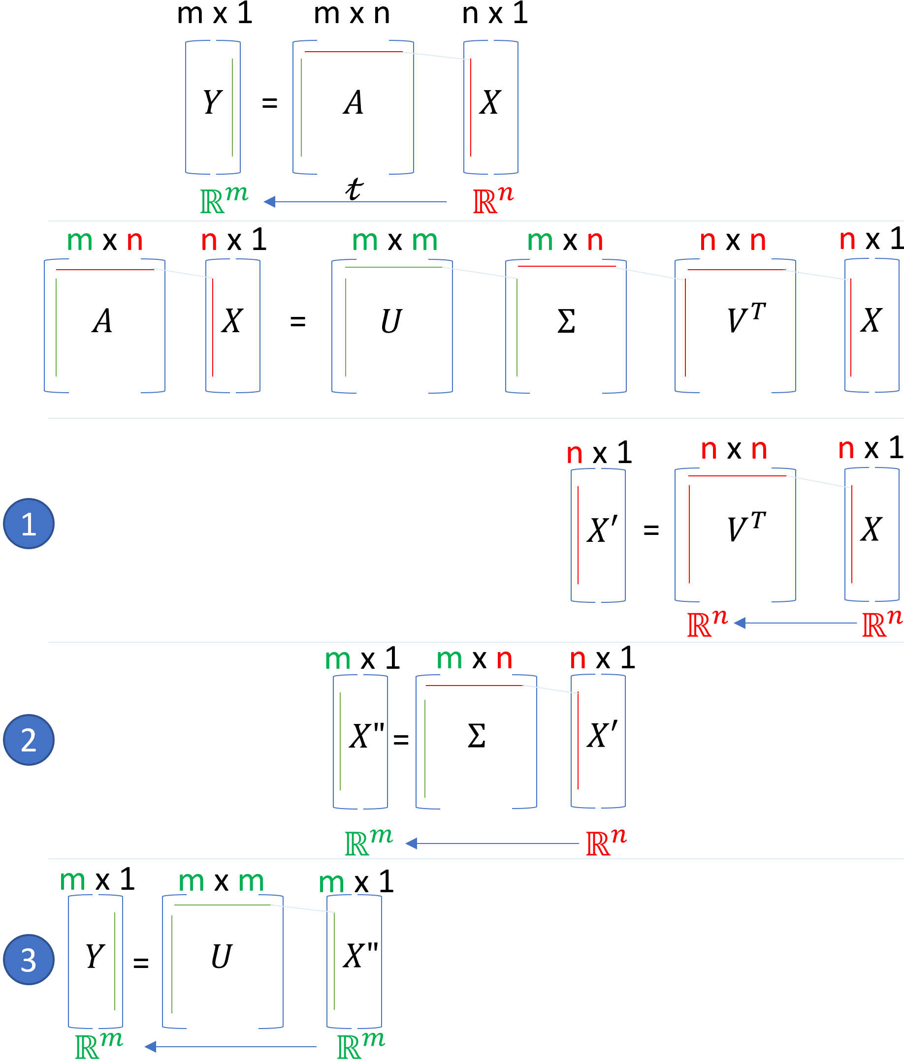
• SVD performs two changes of bases - if you multiply a vector $x\in {\mathbb{R}}^m$ by $U\Sigma V^T$ it will be first transformed into new basis by $V^T$. Then, $\Sigma$ will scale the new coordinates by the singular values (and add/remove some dimensions). Finally, $U$ will perform another base change.
  SVD 包含两次基变换：若向量 $x\in {\mathbb{R}}^m$ 乘以 $U\Sigma V^T$，过程分为三步：首先通过 $V^T$ 将 $x$ 转换到“右奇异向量基”下；然后通过 $\Sigma$（奇异值矩阵）按奇异值缩放新坐标，同时可能增加或减少维度（例如，若 $m>n$，则会从 m 维压缩到n维）；最后通过 $U$ 将结果转换到“左奇异向量基”下（即最终的目标空间基）。

• SVD works both for real and complex matrices, so in general $A=U\Sigma V^{\ast }$, where $V^{\ast }$ is a conjugate transpose of $V$.
  SVD 对实矩阵和复矩阵均适用：对于复矩阵， SVD 的形式为 $A=U\Sigma V^{\ast }$，其中 $V^{\ast }$ 表示 $V$ 的共轭转置（而非普通转置）。

• SVD is a generalisation of a Spectral Decomposition (Eigendecomposition), which is also a diagonal factorisation, but for symmetric matrices only (or, more specifically, Hermitian).
  SVD 是谱分解（Eigendecomposition，即特征值分解）的推广：谱分解也是一种对角化分解，但仅适用于对称矩阵（或更一般的埃尔米特矩阵）；而 SVD 无此限制，可用于任意形状、任意类型（实/复）的矩阵。

• Eigendecomposition (for a square matrix $A$ given by $A=PD{P}^{-1}$), in contrast to SVD , operates in the same vector space (basis change is performed once by $P^{-1}$ and then undone by $P$)
  特征值分解（针对方阵 $A$，形式为 $A=PD{P}^{-1}$）与 SVD 的核心区别在于：特征值分解的两次基变换（$P^{-1}$ 和 $P$）均在同一向量空间中进行（先通过 $P^{-1}$ 换基，经 $D$ 缩放后，再通过 $P$ 换回原基）；而 SVD 的两次基变换（$V^T$ 和 $U$）分别在原空间和目标空间中进行，适用于非方阵的“跨空间变换”。

answered May 27, 2019 at 21:20
Tomasz Bartkowiak
7

The inserted image hopefully adds to the answer of TheSHETTY-Paradise.
插入的图片希望能补充 TheSHETTY-Paradise 的回答（图片展示了 SVD 的三步变换过程）。

It shows the three operations:
图中展示了 SVD 的三个核心操作：
(1) a rotation in the ‘domain’ space,
(1) 在“定义域空间”（domain space，即输入向量所在的空间）中的旋转（对应右奇异向量矩阵 $V$ 的作用）；

(2) a scaling and a change of dimension and then
(2) 缩放与维度变化（对应奇异值矩阵 $\Sigma$ 的作用，奇异值负责缩放，矩阵维度差异实现空间维度的增减）；

(3) a rotation in the image space
(3) 在“像空间”（image space，即输出向量所在的空间）中的旋转（对应左奇异向量矩阵 $U$ 的作用）

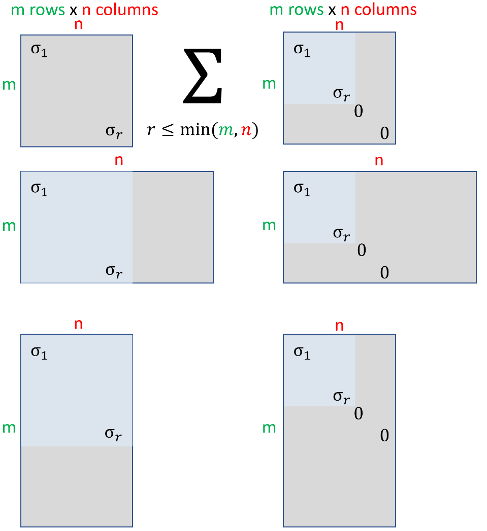
The other image shows all the possible shapes of $\Sigma$
另一张图片则展示了奇异值矩阵 $\Sigma$ 所有可能的形态（例如，针对不同行列数的矩阵 $A$，$\Sigma$ 可能为方阵、“扁长”矩阵或“扁宽”矩阵，但始终是对角矩阵，非对角元素均为0）

answered Nov 30, 2019 at 0:06
Bart Vanderbeke
5

I visualized SVD for myself using the following plot:
我通过以下图表直观理解了 SVD ：（图表通过向量和坐标系展示了 SVD 变换前后的空间变化）

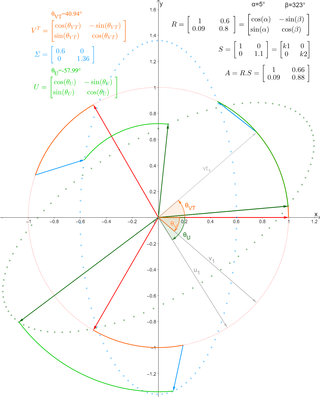
There is a Geogebra app under the link below,
以下链接中有一个 GeoGebra（动态数学软件）应用程序，

you can play around changing the matrix and seeing the effect on the SVD :
你可以通过修改矩阵来实时观察其对 SVD 的影响，奇异值分解可视化

• singular value decomposition visualized
  https://www.heavisidesdinner.com/LTFMfigures/LTFM_figures.html

answered Nov 29, 2019 at 23:23
Bart Vanderbeke
3

Maybe it helps to think in terms of linear transformations rather than matrices. Suppose $V$ and $W$ are finite dimensional inner product spaces over $\mathbb{F}$ (where $\mathbb{F}$ is $\mathbb{R}$ or $\mathbb{C}$) and suppose that $T:V\to W$ is a linear transformation. Then, according to the SVD theorem, there exist orthonormal bases $\alpha$ and $\beta$ (bases of $V$ and $W$, respectively) such that $[T{]}_{\alpha }^{\beta }$ is diagonal.
或许跳出“矩阵”的视角，从“线性变换”的角度理解 SVD 会更容易。假设 $V$ 和 $W$ 是域 $\mathbb{F}$（$\mathbb{F}$ 为实数域 $\mathbb{R}$ 或复数域 $\mathbb{C}$）上的有限维内积空间，$T:V\to W$ 是从 $V$ 到 $W$ 的线性变换。根据 SVD 定理，存在 $V$ 的标准正交基 $\alpha$ 和 $W$ 的标准正交基 $\beta$，使得线性变换 $T$ 在这两组基下的矩阵 $[T{]}_{\alpha }^{\beta }$ 为对角矩阵（即奇异值矩阵 $\Sigma$）。

Trefethen explains a nice geometrical interpretation of the SVD in his book Numerical Linear Algebra.
特雷费森（Trefethen）在其著作《数值线性代数》（Numerical Linear Algebra）中，对 SVD 的几何意义给出了精彩的解释。

answered Aug 26, 2013 at 22:34
littleO
2

There is another geometric interpretation of the singular values of a matrix is the following. Suppose $A$ is an $m\times n$ matrix (real valued, for simplicity). Think of it as a linear transformation ${\mathbb{R}}^n\to {\mathbb{R}}^m$ in the usual way.
矩阵奇异值还有另一种几何解释：假设 $A$ 是 $m\times n$ 实矩阵（为简化，此处限定为实矩阵），按常规方式将其视为从 ${\mathbb{R}}^n$ 到 ${\mathbb{R}}^m$ 的线性变换。

We know from Gauss elimination (see e.g. Gilbert Strang’s book) that the range of the linear mapping $x\to Ax$, which is just the column space. has the same dimension as the row-space of $A$, or better the column-space of $A^{\prime }$ (the transpose (conjugate) matrix), which in turn is the orthogonal complement of the null space of $A$ (because each equation in the homogeneous linear system $A^{\prime }x=0$ refers to orthogonality to one of the row vectors, so the whole system is the same as orthogonality to all the row vectors, which is the same as orthogonality to their linear span (the row space)).
从高斯消元法可知（例如参考吉尔伯特·斯特朗（Gilbert Strang）的著作），线性映射 $x\to Ax$ 的值域（range）就是矩阵 $A$ 的列空间，其维度与 $A$ 的行空间维度相等，也等于转置（或共轭转置）矩阵 $A^{\prime }$ 的列空间维度；而 $A^{\prime }$ 的列空间又是 $A$ 的零空间（null space）的正交补空间——原因是：齐次线性方程组 $A^{\prime }x=0$ 中的每个方程，本质上是“$x$ 与 $A$ 的某一行向量正交”，因此整个方程组等价于“$x$ 与 $A$ 的所有行向量正交”，即“$x$ 与 $A$ 的行空间（行向量的线性张成）正交”。

Usually this is known by the formula: $\text{row rank}(A)=\text{col rank}(A)=:\text{rank}(A)$.
这一性质通常用公式表示为：$\text{行秩}(A)=\text{列秩}(A)=\text{秩}(A)$（矩阵的行秩等于列秩，统称为矩阵的秩）。

So the mapping $x\to Ax$, when restricted to the column-space of $A^{\prime }$ does not have a null space, and thus establishes an isomorphism between the row-space and the column space of $A$.
因此，当线性映射 $x\to Ax$ 的定义域限定为 $A^{\prime }$ 的列空间（即 $A$ 的行空间）时，该映射不存在零空间（即仅当 $x=0$ 时，$Ax=0$），从而在 $A$ 的行空间与列空间之间建立了一个同构关系（isomorphism，即双向唯一、保持线性结构的映射）。

So essentially a matrix $A$ of rank $r$ is in the most general form an isomorphism between two specific $r$-dimensional subspaces of ${\mathbb{R}}^n$ and ${\mathbb{R}}^m$ respectively.
因此，本质上，秩为 $r$ 的矩阵 $A$，其最核心的作用是在 ${\mathbb{R}}^n$ 和 ${\mathbb{R}}^m$ 这两个空间的两个特定 $r$ 维子空间（即 $A$ 的行空间和列空间）之间建立同构。

The remarkable fact then expressed by the SVD theorem is that one can find two orthonormal bases for these two $r$-dimensional spaces such that the linear mapping $x\to Ax$ can be described by a diagonal matrix with non-negative diagonal entries on these spaces. This comes from the spectral theorem applied to the semi-positive matrices $A^{\prime }A$ or $A{A}^{\prime }$.
而 SVD 定理所揭示的惊人事实是：我们可以为这两个 $r$ 维子空间分别找到一组标准正交基，使得线性映射 $x\to Ax$ 在这两组基下的矩阵为“对角元素非负的对角矩阵”（即奇异值矩阵 $\Sigma$）。这一结论的推导，正是基于将“谱定理”（spectral theorem）应用于半正定矩阵 $A^{\prime }A$ 或 $A{A}^{\prime }$（这两个矩阵均满足谱定理的适用条件，可对角化且特征值非负）。

answered May 5, 2016 at 19:19
hgfei
2

Answer referring to Linear Algebra from the book Deep Learning by Ian Goodfellow and 2 others.
本回答参考伊恩·古德费洛（Ian Goodfellow）等三人所著《深度学习》（Deep Learning）一书中的线性代数相关内容。

• The Singular Value Decomposition ( SVD ) provides a way to factorize a matrix, into singular vectors and singular values. Similar to the way that we factorize an integer into its prime factors to learn about the integer, we decompose any matrix into corresponding singular vectors and singular values to understand behaviour of that matrix.
  奇异值分解（ SVD ）提供了一种将矩阵分解为奇异向量和奇异值的方法。这与“将整数分解为质因数以了解整数性质”的思路类似：通过将任意矩阵分解为对应的奇异向量和奇异值，我们可以深入理解矩阵的作用规律。

• SVD can be applied even if the matrix is not square, unlike Eigendecomposition (another form of decomposing a matrix).
  与特征值分解（另一种矩阵分解方法）不同，即使矩阵不是方阵， SVD 也同样适用。

• SVD of any matrix $A$ is given by: $A=UD{V}^T$ (transpose of $V$) The matrix $U$ and $V$ are orthogonal matrices, $D$ is a diagonal matrix (not necessarily square).
  任意矩阵 $A$ 的 SVD 形式为：$A=UD{V}^T$（其中 $V^T$ 表示 $V$ 的转置）。式中，$U$ 和 $V$ 均为正交矩阵，$D$ 为对角矩阵（不一定是方阵）。

• Elements along diagonal $D$ are known as Singular values. The columns of $U$ are known as the left-singular vectors. The columns of $V$ are known as right-singular vectors.
  对角矩阵 $D$ 对角线上的元素称为奇异值；矩阵 $U$ 的列向量称为左奇异向量；矩阵 $V$ 的列向量称为右奇异向量。

• The most useful feature of the SVD is that we can use it to partially generalize matrix inversion to non-square matrices
  SVD 最实用的特性之一是：它能将“矩阵求逆”的概念部分推广到非方阵中（例如，利用 SVD 可以计算非方阵的伪逆，用于解决超定或欠定线性方程组）。

edited Apr 8 at 3:28
Nitin Uniyal
answered Jul 5, 2019 at 10:10
TheSHETTY-Paradise

---

What is the intuition behind SVD?

奇异值分解（SVD）背后的直观理解是什么？

97

I have read about singular value decomposition (SVD). In almost all textbooks it is mentioned that it factorizes the matrix into three matrices with given specification.
我了解过奇异值分解（SVD）。几乎所有教材中都提到，它能将一个矩阵分解为三个具有特定性质的矩阵。

But what is the intuition behind splitting the matrix in such form? PCA and other algorithms for dimensionality reduction are intuitive in the sense that algorithm has nice visualization property but with SVD it is not the case.
但将矩阵分解成这种形式背后的直观逻辑是什么呢？主成分分析（PCA）及其他降维算法的直观性较强，因为这类算法具有良好的可视化特性，而 SVD 却并非如此。

edited May 16, 2020 at 2:39
kjetil b halvorsen♦
asked Oct 15, 2015 at 17:17
SHASHANK GUPTA

• 7
  You might want to start from the intuition of eigenvalue-eigenvector decomposition as SVD is an extension of it for all kinds of matrices, instead of just square ones.
  你可以从特征值 - 特征向量分解的直观理解入手，因为 SVD 是特征值 - 特征向量分解的扩展，它适用于所有类型的矩阵，而不仅仅是方阵。
  –JohnK
  Commented Oct 15, 2015 at 17:43

• 1
  There are plenty of notes on internet and answers here on CV about SVD and its workings.
  互联网上有很多关于 SVD 及其原理的笔记，在 Cross Validated（CV，统计学问答社区）上也有相关答案。
  –Vladislavs Dovgalecs
  Commented Oct 15, 2015 at 17:53

• 3
  SVD can be thought as a compression/learning algorithm. It is a linear compressor decompressor. A matrix M can be represented by multiplication of SVD. S is the compressor V determines how much error you would like to have (lossy compression) and D is the decompressor. If you keep all diagonal values of V then you have a lossless compressor. If you start throwing away small singular values (zeroing them) then you cannot reconstruct the initial matrix exactly but will still be close. Here the term close is measured with Frobenius norm.
  SVD 可被视为一种压缩/学习算法，它是一个线性的压缩 - 解压缩系统。矩阵 M 可以通过 SVD 分解后的矩阵相乘来表示：其中 S 是压缩矩阵，V 决定了期望的误差大小（用于有损压缩），D 是解压缩矩阵。如果保留 V 中所有的对角元素，那么它就是一个无损压缩器；如果舍弃（置零）部分较小的奇异值，就无法精确重建原始矩阵，但重建结果仍会与原始矩阵较为接近——这里的“接近”是通过弗罗贝尼乌斯范数（Frobenius norm）来衡量的。
  –Cagdas Ozgenc
  Commented Oct 15, 2015 at 18:32

• 2
  @Cagdas if you do that please carefully define what you’re taking “S” “V” and “D” to be mathematically. I’ve not seen the initials overloaded into the notation itself before (which has the singular values in it, for example?). It seems to be a likely source of confusion,
  @卡加达斯（Cagdas），如果你采用这种表述，建议从数学上明确“S”“V”和“D”的定义。我此前从未见过用这些首字母来重载 SVD 标准符号的情况（比如，你提到的 V 中包含奇异值，但在标准 SVD 符号中并非如此），这种表述很可能引发混淆。
  –Glen_b
  Commented Oct 15, 2015 at 21:46

• 3
  Do you know how to estimate PCA with SVD? If you do, then can you explain why you feel that something missing in your understanding of SVD? See this
  你知道如何用 SVD 来实现 PCA 吗？如果知道，能否解释一下为什么你觉得自己对 SVD 的理解仍有欠缺？可参考此链接：
  –Aksakal
  Commented Oct 28, 2015 at 16:52

3 Answers

122

Write the SVD of matrix X (real, $n\times p$) as
将矩阵 X（实矩阵，维度为 $n\times p$）的 SVD 分解表示为：

$X=UD{V}^T$

where U is n×p, D is diagonal p×p and $V^T$ is p×p. In terms of the columns of the matrices U and V we can write $X={\sum }_{i=1}^p{d}_i{u}_i{v}_i^T$. That shows X written as a sum of p rank-1 matrices. What does a rank-1 matrix look like? Let’s see:
其中，U 是 n×p 矩阵，D 是 p×p 对角矩阵，$V^T$ 是 p×p 矩阵。从矩阵 U 和 V 的列向量角度，可将 X 表示为 $X={\sum }_{i=1}^p{d}_i{u}_i{v}_i^T$，这表明 X 可分解为 p 个秩为 1 的矩阵之和。那么秩为 1 的矩阵是什么样的呢？请看以下示例：

$\left(\begin{array}{c}1\\ 2\\ 3\end{array}\right)\left(\begin{array}{ccc}4& 5& 6\end{array}\right)=\left(\begin{array}{ccc}4& 5& 6\\ 8& 10& 12\\ 12& 15& 18\end{array}\right)$

The rows are proportional, and the columns are proportional.
该矩阵的所有行向量彼此成比例，所有列向量也彼此成比例。

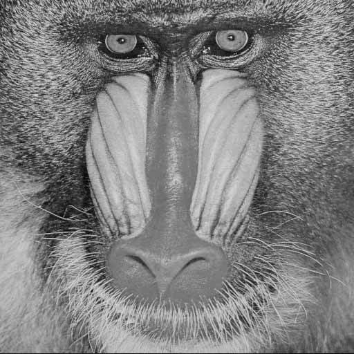
Think now about X as containing the grayscale values of a black-and-white image, each entry in the matrix representing one pixel. For instance the following picture of a baboon:
现在，我们将矩阵 X 视为一张黑白图像的灰度值矩阵——矩阵中的每个元素对应图像的一个像素。例如，以下这张狒狒的图像：

Then read this image into R and get the matrix part of the resulting structure, maybe using the library pixmap.
之后，可使用 R 语言的 pixmap 库将该图像读入，并提取出对应的灰度值矩阵。

If you want a step-by-step guide as to how to reproduce the results, you can find the code here.
若需逐步复现上述结果的操作指南，可在以下链接中获取代码：

Calculate the SVD:
计算该灰度矩阵的 SVD 分解：

baboon.svd  <-  svd (bab) # May take some time

How can we think about this? We get the 512×512 baboon image represented as a sum of 512 simple images, with each one only showing vertical and horizontal structure, i.e. it is an image of vertical and horizontal stripes! So, the SVD of the baboon represents the baboon image as a superposition of 512 simple images, each one only showing horizontal/vertical stripes. Let us calculate a low-rank reconstruction of the image with 1 and with 20 components:
如何理解这一过程？通过 SVD，我们将 512×512 维度的狒狒图像表示为 512 个简单图像的和，且每个简单图像仅包含水平和垂直结构（即由水平和垂直条纹构成）。也就是说，狒狒图像的 SVD 分解，本质是将其分解为 512 个“条纹图像”的叠加。下面我们分别用 1 个和 20 个 SVD 分量来重建低秩图像：

# 第一个成分的重建
baboon.1 <- sweep(baboon.svd$u[, 1, drop = FALSE], 2, baboon.svd$d[1], "*") %*%t(baboon.svd$v[, 1, drop = FALSE])# 前 20 个成分的重建
baboon.20 <- sweep(baboon.svd$u[, 1:20, drop = FALSE], 2, baboon.svd$d[1:20], "*") %*%t(baboon.svd$v[, 1:20, drop = FALSE])

resulting in the following two images:
重建结果如下所示：

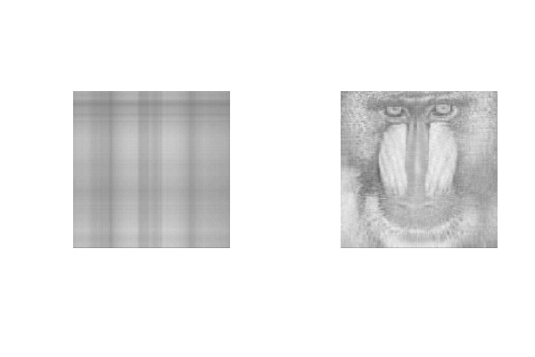
On the left we can easily see the vertical/horizontal stripes in the rank-1 image.
左侧的秩为 1 的重建图像中，可清晰看到水平和垂直条纹。

Let us finally look at the “residual image”, the image reconstructed (as above, code not shown) from the 20 rank-one images with the lowest singular values. Here it is:
最后，我们来看“残差图像”——即使用 20 个具有最小奇异值的秩为 1 矩阵重建得到的图像（重建方法同上，代码未展示），如下所示：

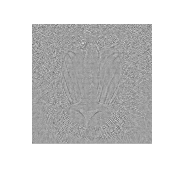
Which is quite interesting: we see the parts of the original image that are difficult to represent as superposition of vertical/horizontal lines, mostly diagonal nose hair and some texture, and the eyes!
这一结果十分有趣：残差图像中呈现的是原始图像中难以用“水平/垂直线条叠加”来表示的部分，主要包括狒狒鼻子上呈对角线分布的毛发、部分纹理结构以及眼睛。

edited Nov 16, 2021 at 15:06
answered Oct 28, 2015 at 13:54
kjetil b halvorsen♦

• 19
  I think you meant low-rank reconstruction, not low range. Never mind. This is a very good illustration (+1). That’s why it is a linear compressor decompressor. Image is approximated with lines. If you actually perform a similar autoencoder with a neural network with linear activation functions, you will actually see that it also allows lines with any slope not only vertical and horizontal lines, which makes it slightly more powerful than SVD.
  我猜你想表达的是“低秩重建（low - rank reconstruction）”而非“低范围重建（low range reconstruction）”，不过这不影响整体理解。这个示例非常好（+1），这也正是 SVD 能作为线性压缩 - 解压缩系统的原因——图像通过线条来近似表示。若用具有线性激活函数的神经网络构建类似的自编码器，你会发现它不仅能处理水平和垂直线条，还能处理任意斜率的线条，因此其功能比 SVD 稍强一些。
  –Cagdas Ozgenc
  Commented Oct 28, 2015 at 14:31

• @kjetil-b-halvorsen Shouldn’t the SVD $X=U\Sigma V^{\ast }$ for a n×p matrix X result in U being n×n, $\Sigma$ being $n\times p$ and V being $p\times p$? Typo?
  @kjetil-b-halvorsen，对于 n×p 矩阵 X，其标准 SVD 分解应为 $X=U\Sigma V^{\ast }$，其中 U 是 $n\times n$ 矩阵，$\Sigma$ 是 $n\times p$ 对角矩阵，V 是 $p\times p$ 矩阵，不是吗？你之前的表述是不是有笔误？
  –Martin Krämer
  Commented Jan 26, 2017 at 17:06

• 3
  See math.StackExchange.com/questions/92171/…for some other examples
  更多相关示例可参考以下链接：
  –kjetil b halvorsen♦
  Commented May 9, 2017 at 10:45

• @kjetil-b-halvorsen I am interested in knowing how would the decription change if I would have used PCA for denosing application. I would appreciate if you could answer my question here
  @kjetil - b - halvorsen，我想知道如果将 PCA 用于去噪任务，上述解释会发生怎样的变化。若你能在以下链接中回答我的问题，我将不胜感激：
  –Dushyant Kumar
  Commented Jun 8, 2019 at 21:31

• @CowboyTrader interesting observation. My understanding of machine learning/neural network is pretty limited. So, I fail to understand that if one has a single noisy image and nothing else to train on, how would the neural network work?
  @CowboyTrader，你的观察很有意思。我对机器学习/神经网络的理解还比较有限，所以不太明白：如果只有一张含噪图像，没有其他数据用于训练，神经网络该如何工作呢？
  –Dushyant Kumar
  Commented Jun 8, 2019 at 21:38

25

Let A be a real m×n matrix. I’ll assume that m≥n for simplicity. It’s natural to ask in which direction v does A have the most impact (or the most explosiveness, or the most amplifying power). The answer is
设 A 为 m×n 实矩阵，为简化分析，假设 m≥n。一个很自然的问题是：在哪个方向向量 v 上，矩阵 A 的“作用最强”（或“放大效应最显著”）？答案如下：

$$\{\begin{array}{l}{v}_1=\arg \underset{v\in {\mathbb{R}}^n}{\max }\Vert Av{\Vert }_2\\ \text{subject to }\Vert v{\Vert }_2=1\end{array}\text{\hspace{1em}(1)}$$

A natural follow-up question is, after $v_1$, what is the next most explosive direction for A? The answer is
接下来的自然问题是：在 $v_1$ 方向之后，矩阵 A 作用第二强的方向是什么？答案是：

$$\{\begin{array}{l}{v}_2=\arg \underset{v\in {\mathbb{R}}^n}{\max }\Vert Av{\Vert }_2\\ \text{subject to }⟨v_1,v⟩=0,\\ \Vert v{\Vert }_2=1\end{array}$$

Continuing like this, we obtain an orthonormal basis $v_1,\dots ,v_n$ of ${\mathbb{R}}^n$. This special basis of ${\mathbb{R}}^n$ tells us the directions that are, in some sense, most important for understanding A.
以此类推，我们可得到 ${\mathbb{R}}^n$ 空间的一组标准正交基 $v_1,\dots ,v_n$。从某种意义上说，这组特殊的基向量揭示了理解矩阵 A 所必需的“关键方向”。

Let ${\sigma }_i=\Vert A{v}_i{\Vert }_2$(so ${\sigma }_i$ quantifies the explosive power of A in the direction $v_i$). Suppose that unit vectors $u_i$ are defined so that
（其中 ${\sigma }_i$ 用于量化矩阵 A 在 $v_i$ 方向上的“放大能力”）。假设单位向量 $u_i$ 满足以下定义：

$$A{v}_i={\sigma }_i{u}_i\text{for }i=1,\dots ,n.\text{\hspace{1em}(2)}$$
The equations (2) can be expressed concisely using matrix notation as
式 (2) 可通过矩阵符号简洁地表示为：

$$AV=U\Sigma ,\text{\hspace{1em}(3)}$$

where V is the n×n matrix whose i-th column is $v_i$, U is the m×n matrix whose i-th column is $u_i$, and $\Sigma$ is the n×n diagonal matrix whose i-th diagonal entry is ${\sigma }_i$. The matrix V is orthogonal, so we can multiply both sides of (3) by $V^T$ to obtain
其中，V 是 n×n 矩阵，其第 i 列为向量 $v_i$；U 是 m×n 矩阵，其第 i 列为向量 $u_i$；$\Sigma$ 是 n×n 对角矩阵，其第 i 个对角元素为 ${\sigma }_i$。由于矩阵 V 是正交矩阵，我们可在式 (3) 两侧同时乘以 $V^T$，得到：

$$A=U\Sigma V^T.$$

It might appear that we have now derived the SVD of A with almost zero effort. None of the steps so far have been difficult. However, a crucial piece of the picture is missing – we do not yet know that the columns of U are pairwise orthogonal.
至此，似乎我们几乎毫不费力地推导出了矩阵 A 的 SVD 分解，上述步骤均不复杂。但关键信息仍有缺失——我们尚未证明矩阵 U 的列向量彼此正交。

Here is the crucial fact, the missing piece: it turns out that $A{v}_1$ is orthogonal to $A{v}_2$:
以下是填补这一空缺的关键结论：$A{v}_1$ 与 $A{v}_2$ 彼此正交，即：

$$⟨A{v}_1,A{v}_2⟩=0.\text{\hspace{1em}(4)}$$

I claim that**if this were not true, then $v_1$ would not be optimal for problem (1).**Indeed, if (4) were not satisfied, then it would be possible to improve $v_1$ by perturbing it a bit in the direction $v_2$.
我认为：若式 (4) 不成立，则 $v_1$ 就不是问题 (1) 的最优解。实际上，若 (4) 不满足，我们只需将 $v_1$ 沿 $v_2$ 方向稍加扰动，就能得到一个“更优”的向量。

Suppose (for a contradiction) that (4) is not satisfied. If $v_1$ is perturbed slightly in the orthogonal direction $v_2$, the norm of $v_1$ does not change (or at least, the change in the norm of $v_1$ is negligible).**When I walk on the surface of the earth, my distance from the center of the earth does not change.**However, when $v_1$ is perturbed in the direction $v_2$, the vector $A{v}_1$ is perturbed in the non-orthogonal direction $A{v}_2$, and so the change in the norm of $A{v}_1$ is non-negligible. The norm of $A{v}_1$ can be increased by a non-negligible amount. This means that $v_1$ is not optimal for problem (1), which is a contradiction. I love this argument because: 1) the intuition is very clear; 2) the intuition can be converted directly into a rigorous proof.
假设（为推出矛盾）式 (4) 不成立。若将 $v_1$ 沿与其正交的 $v_2$ 方向轻微扰动，$v_1$ 的范数不会发生变化（或变化可忽略不计）——这就像“人在地球表面行走时，与地心的距离始终不变”。但当 $v_1$ 沿 $v_2$ 方向扰动时，向量 $A{v}_1$ 会沿 $A{v}_2$ 方向（非正交方向）扰动，因此 $A{v}_1$ 的范数变化不可忽略，甚至可显著增大。这意味着 $v_1$ 并非问题 (1) 的最优解，与假设矛盾。我推崇这一论证，原因有二：1）直观性极强；2）可直接将直观理解转化为严谨证明。

A similar argument shows that $A{v}_3$ is orthogonal to both $A{v}_1$ and $A{v}_2$, and so on. The vectors $A{v}_1,\dots ,A{v}_n$ are pairwise orthogonal. This means that the unit vectors $u_1,\dots ,u_n$ can be chosen to be pairwise orthogonal, which means the matrix U above is an orthogonal matrix. This completes our discovery of the SVD.
通过类似的论证可证明：$A{v}_3$ 与 $A{v}_1$、$A{v}_2$ 均正交，以此类推。最终可得向量 $A{v}_1,\dots ,A{v}_n$ 彼此正交，因此单位向量 $u_1,\dots ,u_n$ 也可选取为彼此正交，即上述矩阵 U 为正交矩阵。至此，我们完整推导并理解了 SVD 分解。

To convert the above intuitive argument into a rigorous proof, we must confront the fact that if $v_1$ is perturbed in the direction $v_2$, the perturbed vector
要将上述直观论证转化为严谨证明，需先解决一个问题：若将 $v_1$ 沿 $v_2$ 方向扰动，得到的扰动向量

$${\tilde{v}}_1=v_1+ϵv_2$$

is not truly a unit vector. (Its norm is $\sqrt{1+{ϵ}^2}$.) To obtain a rigorous proof, define
并非单位向量（其范数为 $\sqrt{1+{ϵ}^2}$）。为严谨起见，我们定义：

$${\bar{v}}_1(ϵ)=\sqrt{1-{ϵ}^2}{v}_1+ϵv_2.$$

The vector ${\bar{v}}_1(ϵ)$ is truly a unit vector. But as you can easily show, if (4) is not satisfied, then for sufficiently small values of $ϵ$ we have
此时，${\bar{v}}_1(ϵ)$ 是标准的单位向量。不难证明：若式 (4) 不成立，则对足够小的 $ϵ$，有

$$f(ϵ)=\Vert A{\bar{v}}_1(ϵ){\Vert }_2^2>\Vert A{v}_1{\Vert }_2^2$$

(assuming that the sign of $ϵ$ is chosen correctly). To show this, just check that $f^{\prime }(0)\ne 0$. This means that $v_1$ is not optimal for problem (1), which is a contradiction.
（只需选取合适符号的 $ϵ$ 即可）。要证明这一点，只需验证 $f^{\prime }(0)\ne 0$。这一结果表明 $v_1$ 并非问题 (1) 的最优解，与原假设矛盾。

(By the way, I recommend reading Qiaochu Yuan’s explanation of the SVD here. In particular, take a look at “Key lemma # 1”, which is what we discussed above. As Qiaochu says, key lemma # 1 is “the technical heart of singular value decomposition”.)
（顺便推荐大家阅读袁翘楚（Qiaochu Yuan）关于 SVD 的解释。尤其建议关注“关键引理 1（Key lemma # 1）”，其内容与我们上述讨论一致。正如袁翘楚所言，该引理是“奇异值分解的技术核心”。）

edited Apr 30, 2020 at 5:42
answered Apr 19, 2019 at 7:52
littleO

• 3
  Love this answer. This is the best way to think about the SVD.
  这个回答太棒了！这是理解 SVD 最直观的方式。
  –Nick Alger
  Commented Nov 26, 2023 at 22:28

• 2
  Fantastic answer! You made my day!
  回答太精彩了！让我豁然开朗！
  –Dagang
  Commented Jan 13, 2024 at 4:58

14

Take an hour of your day and watch this lecture.
建议你花一小时时间观看这个讲座。

• Lecture: The Singular Value Decomposition (SVD) - YouTube
  https://www.youtube.com/watch?v=EokL7E6o1AE

This guy is super straight-forward; It’s important not to skip any of it because it all comes together in the end. Even if it might seem a little slow at the beginning, he is trying to pin down a critical point, which he does!
主讲人讲解非常直白易懂，建议全程观看，因为所有内容最终会串联成一个完整的逻辑体系。即便开头节奏看似稍慢，他也是在为阐明关键知识点做铺垫，且最终效果很好！

I’ll sum it up for you, rather than just giving you the three matrices that everyone does (because that was confusing me when I read other descriptions). Where do those matrices come from and why do we set it up like that? The lecture nails it ! Every matrix (ever in the history of everness) can be constructed from a base matrix with same dimensions, then rotate it, and stretch it (this is the fundamental theorem of linear algebra). Each of those three matrices people throw around represent an initial matrix (U), A scaling matrix (sigma), and a rotation matrix (V).
我会为你总结核心逻辑，而非像其他资料那样只罗列三个分解矩阵（我之前读其他解释时，仅看矩阵分解式就很困惑）。这些矩阵究竟源自何处？为何要这样定义分解形式？讲座给出了清晰答案：历史上所有矩阵，都可由一个同维度的“基础矩阵”通过旋转（rotation）和拉伸（stretching）操作得到（这一思想与线性代数基本定理一致）。人们常提及的 SVD 三个分解矩阵，分别对应：初始矩阵（U）、缩放矩阵（$\Sigma$，即 sigma）和旋转矩阵（V）。

The scaling matrix shows you which rotation vectors are dominating, these are called the singular values. The decomposition is solving for U, sigma, and V.
其中，缩放矩阵 $\Sigma$ 揭示了“哪些旋转方向的作用占主导”——这些主导方向对应的缩放系数就是奇异值（singular values）。而 SVD 分解的本质，就是求解出这三个矩阵 U、$\Sigma$ 和 V。

edited Jun 26, 2021 at 18:39
answered Apr 18, 2019 at 23:40
Tim Johnsen

• Another useful lecture:
  另一个实用的讲座推荐：

  • ME 565 Lecture 27: SVD Part 1 - YouTube
    https://YouTube.com/watch?v=yA66KsFqUAE

  –smile

---

Why are singular values always non-negative?

为什么奇异值始终是非负的？

I have read that the singular values of any matrix $A$ are non-negative (e.g. wikipedia). Is there a reason why?
我了解到任意矩阵 $A$ 的奇异值都是非负的（例如维基百科），这背后是否存在特定原因？

The first possible step to get the SVD of a matrix $A$ is to compute $A^{T}A$. Then the singular values are the square root of the eigenvalues of $A^{T}A$. The matrix $A^{T}A$ is a symmetric matrix for sure. The eigenvalues of symmetric matrices are always real. But why are the eigenvalues (or the singular values) in this case always non-negative as well?
求解矩阵 $A$ 奇异值分解（SVD）的第一步通常是计算 $A^{T}A$，随后奇异值便是 $A^{T}A$ 特征值的平方根。可以确定的是，$A^{T}A$ 是对称矩阵，而对称矩阵的特征值必然是实数，但为何在这种情况下，这些特征值（或由此得到的奇异值）也始终是非负的呢？

asked Dec 15, 2016 at 23:25
Louis

4 Answers

25

Assume that $A$ is real for simplicity. The set of (orthogonal, diagonal, orthogonal) matrices $(U,\Sigma ,V)$ such that $A=U\Sigma V^T$ is not a singleton. Indeed, if $A=U\Sigma V^T$ then also
为简化分析，假设矩阵 $A$ 为实矩阵。满足 $A=U\Sigma V^T$ 的（正交矩阵、对角矩阵、正交矩阵）三元组 $(U,\Sigma ,V)$ 并非唯一。实际上，若 $A=U\Sigma V^T$，则以下形式同样成立：

$A=(-U)(-\Sigma )V^T=U(-\Sigma )(-V^T)=(U{D}_1)(D_1\Sigma D_2)(V{D}_2{)}^T$

for any diagonal matrices $D_1$ and $D_2$ with only $1$ or $-1$ on the diagonal. Therefore, the positivity of the singular values is purely conventional.
其中，$D_1$ 和 $D_2$ 为任意对角线上仅含 $1$ 或 $-1$ 的对角矩阵。因此，奇异值的正性本质上是一种约定俗成的规定。

edited Feb 7, 2024 at 17:57
answered Oct 20, 2019 at 16:42
Roberto Rastapopoulos

19

I’m assuming that the matrix $A$ has real entries, or else you should be considering $A^{\ast }A$ instead.
我假设矩阵 $A$ 为实矩阵；若 $A$ 为复矩阵，则需将后续分析中的 $A^{T}A$ 替换为 $A^{\ast }A$（$A^{\ast }$ 表示 $A$ 的共轭转置）。

If $A$ has real entries then $A^{T}A$ is positive semidefinite, since
若 $A$ 为实矩阵，则 $A^{T}A$ 是半正定矩阵，原因如下：对任意向量 $v$，均有

$⟨A^{T}Av,v⟩=⟨Av,Av⟩\ge 0$

for all $v$. Therefore the eigenvalues of $A^{T}A$ are non-negative.
$⟨A^{T}Av,v⟩=⟨Av,Av⟩\ge 0$（内积的非负性）。因此，$A^{T}A$ 的特征值必然是非负的。

answered Dec 15, 2016 at 23:30
carmichael561

• 11
  This shows that the eigenvalues of $A^{T}A$ are non-negative, what about the singular values of $A$? Do you know if the fact that the singular values of $A$ are (non-negative) square roots of the eigenvalues of $A^{H}A$ holds for $A$ with complex entries?
  这证明了 $A^{T}A$ 的特征值是非负的，但矩阵 $A$ 的奇异值呢？对于复矩阵 $A$，其奇异值是 $A^{H}A$（$A^H$ 为 $A$ 的共轭转置）特征值的（非负）平方根，这一结论是否仍然成立？

  – Learn_and_Share
  Commented Oct 25, 2017 at 8:42

• Yes, the singular values of $A$ are the square roots of the eigenvalues of $A^{\ast }A$.

  是的，无论 $A$ 是实矩阵还是复矩阵，其奇异值都是 $A^{\ast }A$（实矩阵中 $A^{\ast }=A^T$，复矩阵中 $A^{\ast }$ 为共轭转置）特征值的平方根。
  ——卡迈克尔 561（carmichael561）

  – carmichael561
  Commented Oct 25, 2017 at 15:11

• 7
  @MedNait Why are they chosen to be the positive square roots?
  @MedNait，为什么要选择特征值的正平方根作为奇异值呢？

  – Undertherainbow
  Commented Feb 19, 2018 at 15:25

• 6
  @Undertherainbow I think I read somewhere that it’s a convention since, technically, you could also choose the singular values of $A$ as the negative square roots of the eigenvalues of $A^{H}A$.
  @彩虹之下（Undertherainbow），我记得曾在某处看到过相关解释：这本质上是一种约定。从技术角度而言，理论上也可以将 $A$ 的奇异值定义为 $A^{H}A$ 特征值的负平方根，但行业内普遍采用正平方根的定义。

  – Learn_and_Share
  Commented Feb 19, 2018 at 20:50

6

I think your question is very interesting. Let us take some, non zero singular value ${\sigma }_i$. We can reverse the sign if it is positive. That is, $-{\sigma }_i=-\sqrt{{\lambda }_i^2}=-{\lambda }_i$ where ${\lambda }_i^2$ is an eigenvalue of $A^{T}A$ corresponding to an eigenvector $v_i$. That is $A^{T}A{v}_i={\lambda }_i^2{v}_i$. Who can stop us to write instead $A^{T}A(-v_i)={\lambda }_i^2(-v_i)$? What this means is that we can reverse the sign of a singular value, but then we need to go to the matrix $V$ and reverse the sign of its corresponding eigenvector column.
我认为你的问题非常有意思。假设存在一个非零奇异值 ${\sigma }_i$，即便它是正数，我们理论上也可以改变其符号——即 $-{\sigma }_i=-\sqrt{{\lambda }_i^2}=-{\lambda }_i$，其中 ${\lambda }_i^2$ 是 $A^{T}A$ 对应于特征向量 $v_i$ 的特征值（满足 $A^{T}A{v}_i={\lambda }_i^2{v}_i$）。既然 $A^{T}A(-v_i)={\lambda }_i^2(-v_i)$（$-v_i$ 同样是 $A^{T}A$ 对应于 ${\lambda }_i^2$ 的特征向量），那么为什么不能将奇异值定义为 $-{\lambda }_i$ 呢？这一现象表明：我们确实可以改变某个奇异值的符号，但与此同时，必须同步改变矩阵 $V$ 中对应特征向量列的符号。

Hence, there is not a unique way to write $A=U\Sigma V^T$. But if we decide that all ${\sigma }_i$ are non-negative, then “yes” there is a unique way to write $A=U\Sigma V^T$. Of course all ${\sigma }_i$ are sorted from largest to smallest (otherwise there would be a bunch of possibilities by permuting any two columns of $U$ and $V$ and their corresponding eigenvalues.)
因此，$A=U\Sigma V^T$ 的分解形式并非唯一。但如果我们约定所有奇异值 ${\sigma }_i$ 均为非负，那么 $A=U\Sigma V^T$ 的分解形式就具有了唯一性（通常还会约定奇异值按从大到小的顺序排列；否则，交换 $U$ 和 $V$ 中任意两列的位置及对应奇异值，会产生更多分解形式）。

edited Jul 29, 2019 at 22:29
answered Jul 29, 2019 at 22:05
Herman Jaramillo

5

Suppose $T\in \mathcal{L}(V)$, i.e., $T$ is a linear operator on the vector space $V$. Then the singular values of $T$ are the eigenvalues of the positive operator $\sqrt{T^{\ast }T}$. The eigenvalues of a positive operator are non-negative.
假设 $T\in \mathcal{L}(V)$（即 $T$ 是向量空间 $V$ 上的线性算子），则 $T$ 的奇异值定义为正算子 $\sqrt{T^{\ast }T}$ 的特征值。而正算子的特征值必然是非负的，具体推导如下：

• Why is $\sqrt{T^{\ast }T}$ a positive operator? Consider $S=T^{\ast }T$. Then $S^{\ast }=(T^{\ast }T{)}^{\ast }=T^{\ast }(T^{\ast }{)}^{\ast }=T^{\ast }T=S$, and hence $S$ is self-adjoint. Also, $⟨Sv,v⟩=⟨T^{\ast }Tv,v⟩=⟨Tv,Tv⟩\ge 0$ for every $v\in V$. Hence $S$ is positive. Now every positive operator has a unique positive square root, which, for $S$, I am denoting with $\sqrt{T^{\ast }T}$.

  为什么 $\sqrt{T^{\ast }T}$ 是正算子？令 $S=T^{\ast }T$，则 $S^{\ast }=(T^{\ast }T{)}^{\ast }=T^{\ast }(T^{\ast }{)}^{\ast }=T^{\ast }T=S$，即 $S$ 是自伴算子（自共轭算子）。此外，对任意 $v\in V$，均有 $⟨Sv,v⟩=⟨T^{\ast }Tv,v⟩=⟨Tv,Tv⟩\ge 0$（内积的非负性），因此 $S$ 是正算子。而每个正算子都存在唯一的正平方根，这里 $S=T^{\ast }T$ 的正平方根记为 $\sqrt{T^{\ast }T}$。

• Why are the eigenvalues of a positive operator non-negative? If $S$ is a positive operator, then $0\le ⟨Sv,v⟩=⟨\lambda v,v⟩=\lambda ⟨v,v⟩$, and thus $\lambda$ is non-negative.

  为什么正算子的特征值是非负的？若 $S$ 是正算子，对其任意特征值 $\lambda$ 及对应特征向量 $v$，有 $0\le ⟨Sv,v⟩=⟨\lambda v,v⟩=\lambda ⟨v,v⟩$。由于 $⟨v,v⟩>0$（特征向量非零），因此 $\lambda \ge 0$。

answered Apr 21, 2019 at 6:35
Aditya

---

via：

• linear algebra - Why is the SVD named so?
  https://math.stackexchange.com/questions/360214/why-is-the-SVD-named-so

• linear algebra - Understanding the singular value decomposition ( SVD )
  https://math.stackexchange.com/questions/411486/understanding-the-singular-value-decomposition-SVD

• What is the intuition behind SVD ?
  https://stats.stackexchange.com/questions/177102/what-is-the-intuition-behind-SVD/403924

• svd - Why are singular values always non-negative? - Mathematics Stack Exchange
  https://math.stackexchange.com/questions/2060572/why-are-singular-values-always-non-negative