CS231n学习笔记3-3: DDPM

作业三-Q3: Denoising Diffusion Probabilistic Models(DDPM)

作业流程

本节任务

• 理解 DDPM 框架的图片生成原理和架构，以及下面的几个子步骤
• 理解 UNet 模型的结构并完成对应的 Block
• 完成损失函数 p_losses 的设计
• 理解反向去噪的原理并完成 p_sample
• 理解调控条件影响强度的 CFG 方法
• 对表情生成任务进行模型训练和采样

准备

在 conda 环境中补充几个包:

pip install joblib einops

代码详解

1. DDPM 生成框架

原论文链接: https://arxiv.org/pdf/2006.11239

可以观看 b 站上的讲解视频以加深理解：https://www.bilibili.com/video/BV1tz4y1h7q1

作业中对 DDPM 的描述：

去噪扩散概率模型（DDPM）

到目前为止，我们讨论的都是判别式模型，它们被训练来输出带标签的结果。从基础的图像分类，到以分类为框架的句子生成（在词表空间进行分类，并用递归机制捕获多词标签），都属于这一类。现在，我们将扩展工具箱，构建一种生成式模型，能够根据给定的训练图像集合生成逼真的新图像。

生成模型有很多类型，包括生成对抗网络（GAN）、自回归模型、可逆流（Normalizing Flow）模型以及变分自编码器（VAE）等，它们都能合成效果出色的图像。然而，2020 年 Ho 等人将扩散概率模型与去噪分数匹配相结合，提出了去噪扩散概率模型（DDPM）。这一模型既易于训练，又足以生成复杂、高质量的图像。以下给出 DDPM 的高层概述。更多细节请参考课程讲义与原始论文。

正向过程（Forward Process）
设 $q(x_0)$ 为干净数据图像的分布。定义一个逐步加噪的马尔可夫链：

$$q(x_t\mid x_{t-1})\sim \mathcal{N}(x_t;\sqrt{1-{\beta }_t}{x}_{t-1},{\beta }_{t}I),$$

其中逐步方差序列 $({\beta }_1,\dots ,{\beta }_T)$ 决定了噪声日程（noise schedule）。利用高斯分布的性质，可以得到封闭形式的

$$q(x_t\mid x_0)\sim \mathcal{N}(x_t;\sqrt{{\bar{\alpha }}_t}{x}_0,(1-{\bar{\alpha }}_t)I),$$

其中 ${\alpha }_t=1-{\beta }_t$，${\bar{\alpha }}_t={\prod }_{s=1}^t{\alpha }_s$。如果噪声日程 $({\beta }_1,\dots ,{\beta }_T)$ 设定得当，最终分布 $q(x_T)$ 将与标准高斯噪声 $\mathcal{N}(0,I)$ 几乎不可区分。

回忆一下，从高斯分布 $x\sim \mathcal{N}(\mu ,{\sigma }^2)$ 采样等价于计算 $\sigma \cdot ϵ+\mu$，其中 $ϵ\sim \mathcal{N}(0,1)$。因此，给定 $x_{t-1}$ 或 $x_0$，从 $q(x_t\mid x_{t-1})$ 或 $q(x_t\mid x_0)$ 采样都是直接、简单且无需学习的。

逆向过程（Reverse Process）
逆向过程从纯噪声 $x_T$ 通过多步重建干净图像 $x_0$。令 $p(x_{t-1}\mid x_t)$ 表示 $q(x_t\mid x_{t-1})$ 的逆过程一步。第一个关键洞见是：逐步学习每个去噪步骤要比一次性学习整个正向过程的逆过程容易。也就是说，分别学习每个 $t$ 的 $p(x_{t-1}\mid x_t)$，要比直接学习 $p(x_0\mid x_T)$ 更容易。

但学习 $p(x_{t-1}\mid x_t)$ 仍然具有挑战。尽管 $q(x_t\mid x_{t-1})$ 是高斯分布，$p(x_{t-1}\mid x_t)$ 却可能是任意复杂的分布，几乎肯定不是高斯。刻画并从任意分布采样远比处理参数化的高斯分布要困难。

第二个关键洞见是：如果正向过程中的每一步噪声 ${\beta }_t$ 足够小，那么逆向一步 $p(x_{t-1}\mid x_t)$ 也会接近高斯分布。因此，我们只需估计其均值和方差。在实践中，将 $p(x_{t-1}\mid x_t)$ 的方差固定为与正向相关的小常数（例如固定为 ${\beta }_t$，或采用论文中的 ${\tilde{\beta }}_t$ 设定）通常效果良好。于是，学习逆向过程可简化为学习其均值 $\mu (x_t,t;\theta )$，其中 $\theta$ 是神经网络的参数。

去噪目标（Denoising Objective）
生成模型通常通过最小化数据样本的期望负对数似然 $\mathbb{E}[-\log p_{\theta }(x_0)]$ 来优化。每个样本的似然可写为

$$p_{\theta }(x_0)=p(x_T)\prod _{t=1}^{T}p(x_{t-1}\mid x_t).$$

由于该目标在许多情况下难以直接优化，通常改为优化其变分下界（ELBO）。

Ho 等人进一步展示：在固定方差等设定下，训练可等价地采用一个更简单的去噪损失（常称“简化目标”）：

$${\mathbb{E}}_{t,x_0,ϵ}[\Vert ϵ-{ϵ}_{\theta }(\sqrt{{\bar{\alpha }}_t}{x}_0+\sqrt{1-{\bar{\alpha }}_t}ϵ,t\left){\Vert }^2\right],$$

其中 $t$ 在 $\mathrm{1..}T$ 间均匀采样，$x_0$ 是干净样本，$ϵ\sim \mathcal{N}(0,I)$，而 ${ϵ}_{\theta }$ 是训练来从带噪输入 $x_t=\sqrt{{\bar{\alpha }}_t}{x}_0+\sqrt{1-{\bar{\alpha }}_t}ϵ$ 预测噪声 $ϵ$ 的神经网络。换言之，${ϵ}_{\theta }$ 学习对输入的噪声图像进行去噪。注意，这与预测干净样本在信息上是等价的，因为由上式可由 $(x_t,x_0)$ 恢复出噪声 $ϵ$。

Implementation1: q_sample() & predict_start_from_noise() & predict_noise_from_start()

首先我们先引出一个重要公式。给定原始样本 (x_0)，经过 (t) 次高斯噪声注入后得到的 (x_t) 仍然是高斯分布. 记 (\alpha_t := 1-\beta_t)，(\bar\alpha_t := \prod_{s = 1}^t \alpha_s), 用标准高斯噪声 (\varepsilon\sim\mathcal N(0, I)) 表示, 得到以下公式(1)：

$$x_t=\sqrt{{\bar{\alpha }}_t}{x}_0+\sqrt{1-{\bar{\alpha }}_t}\epsilon \text{\hspace{1em}(1)}$$

按照该公式完成三个函数。q_sample 函数的目的是通过初始图片和采样得到的噪声生成时间步 t 之后的噪声图片。是从清晰到混乱的正向过程。

已知初始图片 x0，时间步 t，噪声 noise，累计信号保留率 alphas_cumprod，计算 t 时间步后的图片 xt。

q_sample 代码如下:

    def q_sample(self, x_start, t, noise):"""Sample from q(x_t | x_0) according to Eq. (4) of the paper.Args:x_start: (b, *) tensor. Starting image.t: (b,) tensor. Time step.noise: (b, *) tensor. Noise from N(0, 1).Returns:x_t: (b, *) tensor. Noisy image."""x_t = None##################################################################### TODO:# Implement sampling from q(x_t | x_0) according to Eq. (4) of the paper.# Hints: (1) Look at the `__init__` method to see precomputed coefficients.# (2) Use the `extract` function defined above to extract the coefficients# for the given time step `t`. (3) Recall that sampling from N(mu, sigma^2)# can be done as: x_t = mu + sigma * noise where noise is sampled from N(0, 1).# Approximately 3 lines of code.####################################################################x_start_param = extract(self.sqrt_alphas_cumprod, t, x_start.shape)noise_param = extract(self.sqrt_one_minus_alphas_cumprod, t, x_start.shape)x_t = x_start_param * x_start + noise_param * noise####################################################################return x_t

predict_start_from_noise() & predict_noise_from_start() 函数同样也是基于公式(1)的逻辑，目的是在已知噪声图片的情况下, 初始图片和噪声已知其一求另一个。因此构建输入为噪声图片的反向预测的模型时，只需要预测噪声就可以求得初始图片。

predict_start_from_noise 和 predict_noise_from_start 代码如下:

    def predict_start_from_noise(self, x_t, t, noise):"""Get x_start from x_t and noise according to Eq. (14) of the paper.Args:x_t: (b, *) tensor. Noisy image.t: (b,) tensor. Time step.noise: (b, *) tensor. Noise from N(0, 1).Returns:x_start: (b, *) tensor. Starting image."""x_start = None##################################################################### TODO:# Transform x_t and noise to get x_start according to Eq.(4) and Eq.(14).# Look at the coeffs in `__init__` method and use the `extract` function.####################################################################x_start_param = extract(self.sqrt_alphas_cumprod, t, x_t.shape)noise_param = extract(self.sqrt_one_minus_alphas_cumprod, t, x_t.shape)x_start = (x_t - noise_param * noise) / x_start_param####################################################################return x_startdef predict_noise_from_start(self, x_t, t, x_start):"""Get noise from x_t and x_start according to Eq. (14) of the paper.Args:x_t: (b, *) tensor. Noisy image.t: (b,) tensor. Time step.x_start: (b, *) tensor. Starting image.Returns:pred_noise: (b, *) tensor. Predicted noise."""pred_noise = None##################################################################### TODO:# Transform x_t and noise to get x_start according to Eq.(4) and Eq.(14).# Look at the coeffs in `__init__` method and use the `extract` function.####################################################################x_start_param = extract(self.sqrt_alphas_cumprod, t, x_t.shape)noise_param = extract(self.sqrt_one_minus_alphas_cumprod, t, x_t.shape)pred_noise = (x_t - x_start_param * x_start) / noise_param####################################################################return pred_noise

2. UNet 模型

我们使用 UNet 模型去噪。

UNet-模型结构图

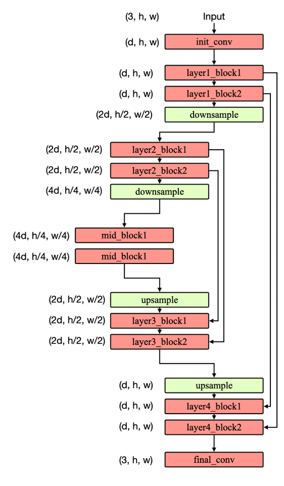
UNet-模型概述

UNet 采用对称的编码器—解码器结构。编码端由若干阶段的卷积块组成，每下采样一次，空间分辨率依次从(h, w)降为(h/2, w/2)、(h/4, w/4)，同时通道数从 d 增至 2d、4d，用以提取更具语义的特征。网络在最低分辨率处设瓶颈块以聚合全局上下文。解码端逐级上采样，通道数相应减半，并在每个尺度与编码端同尺度的特征通过跳跃连接进行融合（通常在通道维拼接），随后再经卷积块细化重建。最后通过一层卷积将特征映射到目标通道数，输出与输入分辨率一致的结果。

该结构的核心在于在恢复空间细节的同时利用跳跃连接保留低层的边缘与纹理信息，从而实现精确的像素级预测。其主要作用是进行语义分割等密集预测任务，在样本规模有限的情况下也能取得稳定而准确的结果。

相关概念解释:

一、什么是瓶颈块
在 UNet 中，瓶颈块位于编码器与解码器之间、空间分辨率最低的一层。其作用是在最小的 h×w 上用较高的通道数聚合全局上下文，通常由两到数个卷积块（如 3×3 卷积 + 归一化 + 激活，可能带 Dropout 或空洞卷积）组成。这里的“瓶颈”强调的是位于网络中部、空间尺度最小而语义最强。

二、为什么降采样与升采样时常伴随通道数改变
降采样后，空间元素变少但语义更抽象，通常将通道数按阶段翻倍以提升表示容量，并在总体计算上保持近似平衡。卷积的主导计算量近似为 H·W·C_in·C_out·k^2；当 H、W 各减半时，将 C_out 约翻倍可使计算量与内存占用保持在可控水平，同时扩大感受野与特征通道的表达力。解码阶段则镜像地将分辨率上采样、通道数减半，以便在恢复细节的同时控制计算量，并与编码端的跳跃特征在通道维拼接后再用卷积整合。

需要区分：插值式上采样本身不改变通道数，通道的变化通常由紧随其后的卷积（或转置卷积本身）完成；降采样亦然，最大池化不改通道，步幅卷积会同时变更空间与通道。

三、拼接后的维度
UNet 的跳跃连接在通道维进行拼接，要求两支的空间尺寸一致。举例来讲，若一支为 (B, 2d, h/2, w/2)，另一支也是 (B, 2d, h/2, w/2)，拼接后张量为 (B, 4d, h/2, w/2)。随后常用卷积将通道数压回解码器该层的目标通道（如 2d），完成特征融合。经典 UNet（valid 卷积）会对跳跃分支做裁剪以匹配尺寸；现代实现多用 same padding，避免裁剪。

四、上采样与下采样的常见实现

下采样：

1. 2×2 最大池化或平均池化，步幅 2，仅改变空间尺寸；随后用卷积调整通道数。
2. 步幅卷积（如 3×3，stride 2，padding 1），同时完成降采样与通道变换，语义更强。
3. 可选的抗混叠变体（如 blur pooling）以减轻混叠与位移不变性问题。

上采样：

1. 双线性或最近邻插值上采样 2 倍，随后用 3×3 卷积细化并调通道，稳定且无栅格伪影。
2. 转置卷积（如 kernel 2、stride 2 或 kernel 4、stride 2），一次性学习性地放大并改通道，但需要注意网格伪影，可配合合适的核与初始化。
3. 像素重排（pixel shuffle）等方法也可用于特定场景。

五、DDPM 与 U‑Net 的关系

DDPM 是整体生成框架，定义了前向加噪与逆向去噪的概率过程，以及基于随机时刻监督的训练目标。U‑Net 是具体的神经网络结构，完成 ${\epsilon }_{\theta }(x_t,t,c)$ 的函数近似过程。

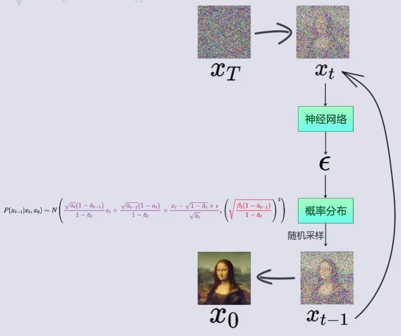
(图片截自 B 站视频)

---

UNet-Down Block&Up Block

概述：

首先 UNet 的主干部分就是 Downsampling Block & Upsampling Block。每个 Downsampling Block & Upsampling Block 里面都包含着 Resnet Block&Down/Upsample。

Downsampling Block = [Resnet Block(dim_in→dim_in) → Resnet Block(dim_in→dim_in) → Downsample(dim_in→dim_out)]

Resnet Block = [[Conv(d_in→d_out) → Norm → Act] → Dropout → [Conv(d_out→d_out) → Norm → Act] → Add]

Downsample = [Conv(d_in, d_out, 2, 2)]

Upsampling Block = [Upsample(dim_in, dim_out) (cat(k)) → Resnet Block(2 * dim_out → dim_out) (cat(k-1)) → Resnet Block(2 * dim_out → dim_out)]

Upsample = [bilinear ↑2 → Conv(d_in, d_out, 3, 1)]

cat(k) := cat([·, skip_k], dim = 1) （拼接是张量操作，放在 forward 里完成。拼接维度是通道维度。）

Resnet Block 结构同上。

代码实现：

Up&Down Block 在代码中的实现如下：

for ind, (dim_in, dim_out) in enumerate(in_out):down_block = nn.ModuleList([ResnetBlock(dim_in, dim_in, context_dim),ResnetBlock(dim_in, dim_in, context_dim),Downsample(dim_in, dim_out),])self.downs.append(down_block)for ind, (dim_in, dim_out) in enumerate(in_out_ups):up_block = nn.ModuleList([Upsample(dim_in, dim_out),ResnetBlock(2*dim_out, dim_out, context_dim),ResnetBlock(2*dim_out, dim_out, context_dim),])self.ups.append(up_block)

在构建 Up&Down Block 的时候需要使用到 ResnetBlock 以及 ResnetBlock 中的 Block（Conv+RESNorm+GELU）。这个过程同时也包括了 context 传入 Up&Down Block 后经过一系列变化得到 scale 和 shift 并嵌入特征的过程。context 不随 block 的变化而变化，同一时间步自始至终都一致。

Block 和 ResnetBlock 代码如下：

class Block(nn.Module):"""A conv block with feature modulation."""def __init__(self, dim, dim_out):super().__init__()self.proj = nn.Conv2d(dim, dim_out, 3, padding=1)self.norm = RMSNorm(dim_out)self.act = nn.GELU()def forward(self, x, scale_shift=None):x = self.proj(x)x = self.norm(x)# Scale and shift are used to modulate the output. This is a variant# of feature fusion, more powerful than simply adding the feature maps.if exists(scale_shift):scale, shift = scale_shiftx = x * (scale + 1) + shiftx = self.act(x)return x
class ResnetBlock(nn.Module):"""A ResNet-like block with context dependent feature modulation."""def __init__(self, dim, dim_out, context_dim):super().__init__()self.dim = dimself.dim_out = dim_outself.context_dim = context_dimself.mlp = (nn.Sequential(nn.GELU(), nn.Linear(context_dim, dim_out * 2))if exists(context_dim)else None)self.block1 = Block(dim, dim_out)self.block2 = Block(dim_out, dim_out)self.res_conv = nn.Conv2d(dim, dim_out, 1) if dim != dim_out else nn.Identity()self.dropout = nn.Dropout(0.1)def forward(self, x, context=None):scale_shift = Noneif exists(self.mlp) and exists(context):context = self.mlp(context)context = rearrange(context, "b c -> b c 1 1")scale_shift = context.chunk(2, dim=1)h = self.block1(x, scale_shift=scale_shift)h = self.dropout(h)h = self.block2(h)return h + self.res_conv(x)

Unet 模型的整个结构在 Unet 类中的 init 函数中编写。Unet 根据 2 的倍数序列生成对应大小的 Up&Down Block，并构建了处理时间步 t 和条件参数（此处为 text）的 mlp：time_mlp&cond_mlp，也构建了必不可少的 Middle blocks（Resnet Block）以及头尾部分的卷积层 init_conv&final_conv。

Unet 类的 init() 代码如下：

    def __init__(self,dim,condition_dim,dim_mults=(1, 2, 4, 8),channels=3,uncond_prob=0.2,):super().__init__()self.init_conv = nn.Conv2d(channels, dim, 3, padding=1)self.channels = channels# Number of channels at each layer i.e. [d1, d2, ..., dn]dims = [dim] + [dim * m for m in dim_mults]# Input and output for each U-Net block in downsampling layers# e.g. [(d1, d2), (d2, d3), ..., (dn-1, dn)]in_out = list(zip(dims[:-1], dims[1:]))# Input and output for each U-Net block in upsampling layers# e.g. [(dn, dn-1), (dn-1, dn-2), ..., (d2, d1)]in_out_ups = [(b, a) for a, b in reversed(in_out)]# Encoding timestep as contextcontext_dim = dim * 4self.time_mlp = nn.Sequential(SinusoidalPosEmb(dim),nn.Linear(dim, context_dim),nn.GELU(),nn.Linear(context_dim, context_dim),)# Encoding condition (i.e. text embedding) as contextself.condition_dim = condition_dimself.condition_mlp = nn.Sequential(nn.Linear(condition_dim, context_dim),nn.GELU(),nn.Linear(context_dim, context_dim),)# Probability of dropping the condition during trainingself.uncond_prob = uncond_prob# UNet downsampling and upsampling blocks.# self.downs is a ModuleList of ModuleLists.self.downs = nn.ModuleList([])# self.ups is a ModuleList of ModuleLists.self.ups = nn.ModuleList([])##################################################################### Downsampling blocks####################################################################for ind, (dim_in, dim_out) in enumerate(in_out):down_block = None################################################################### TODO: Create one UNet downsampling layer `down_block` as a ModuleList.# It should be a ModuleList of 3 blocks [ResnetBlock, ResnetBlock, Downsample].# Each ResnetBlock operates on dim_in channels and outputs dim_in channels.# Make sure to pass the context_dim to each ResnetBlock.# The Downsample block operates on dim_in channels and outputs dim_out channels.# Make sure to exactly follow this structure of ModuleList in order to# load a pretrained checkpoint.##################################################################down_block = nn.ModuleList([ResnetBlock(dim_in, dim_in, context_dim),ResnetBlock(dim_in, dim_in, context_dim),Downsample(dim_in, dim_out),])##################################################################self.downs.append(down_block)# Middle blocksmid_dim = dims[-1]self.mid_block1 = ResnetBlock(mid_dim, mid_dim, context_dim=context_dim)self.mid_block2 = ResnetBlock(mid_dim, mid_dim, context_dim=context_dim)##################################################################### Upsampling blocks##################################################################### Create upsampling blocks by exactly mirroring the downsampling blocks.# self.ups will also be a ModuleList of ModuleLists.# Each BlockList will contain 3 blocks [Upsample, ResnetBlock, ResnetBlock].for ind, (dim_in, dim_out) in enumerate(in_out_ups):up_block = None################################################################### TODO: Create one UNet upsampling layer as a ModuleList.# It should be a ModuleList of 3 blocks [Upsample, ResnetBlock, ResnetBlock].# This will mirror the corresponding downsampling block.# Don't forget to account for the skip connections by having 2 x dim_out# channels at the input of both ResnetBlocks.##################################################################up_block = nn.ModuleList([Upsample(dim_in, dim_out),ResnetBlock(2*dim_out, dim_out, context_dim),ResnetBlock(2*dim_out, dim_out, context_dim),])##################################################################self.ups.append(up_block)# Final convolution to map to the output channelsself.final_conv = nn.Conv2d(dim, channels, 1)

---

UNet-Forward

Forward 流程图

首先我们通过均匀分布和正态分布分别取样时间步 t 和噪声 noise，并从数据集中读取 x_start，通过这些数据根据公式(1)得到 xt。随后根据 t 和 text 得到 context。

做好数据准备后，构建 Block -> RESBlock+Up/Downsampling Block -> Up/Down Block -> UNet model。

最后将 xt 和 context 传入 UNet model，得到噪声的预测值。

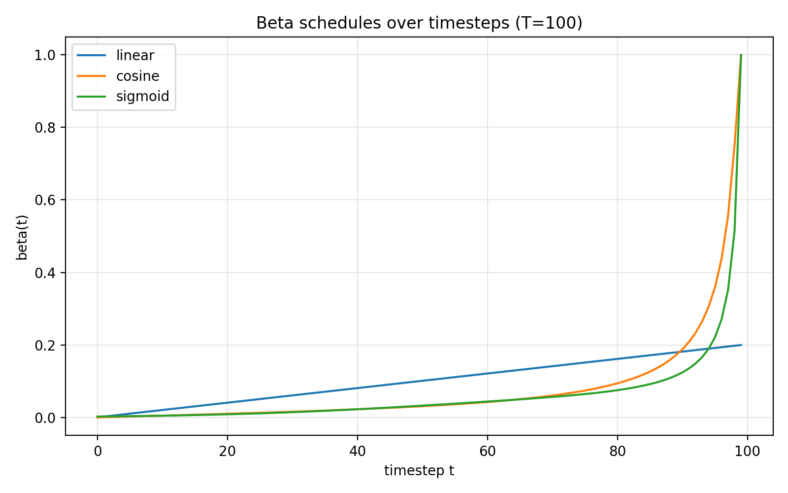
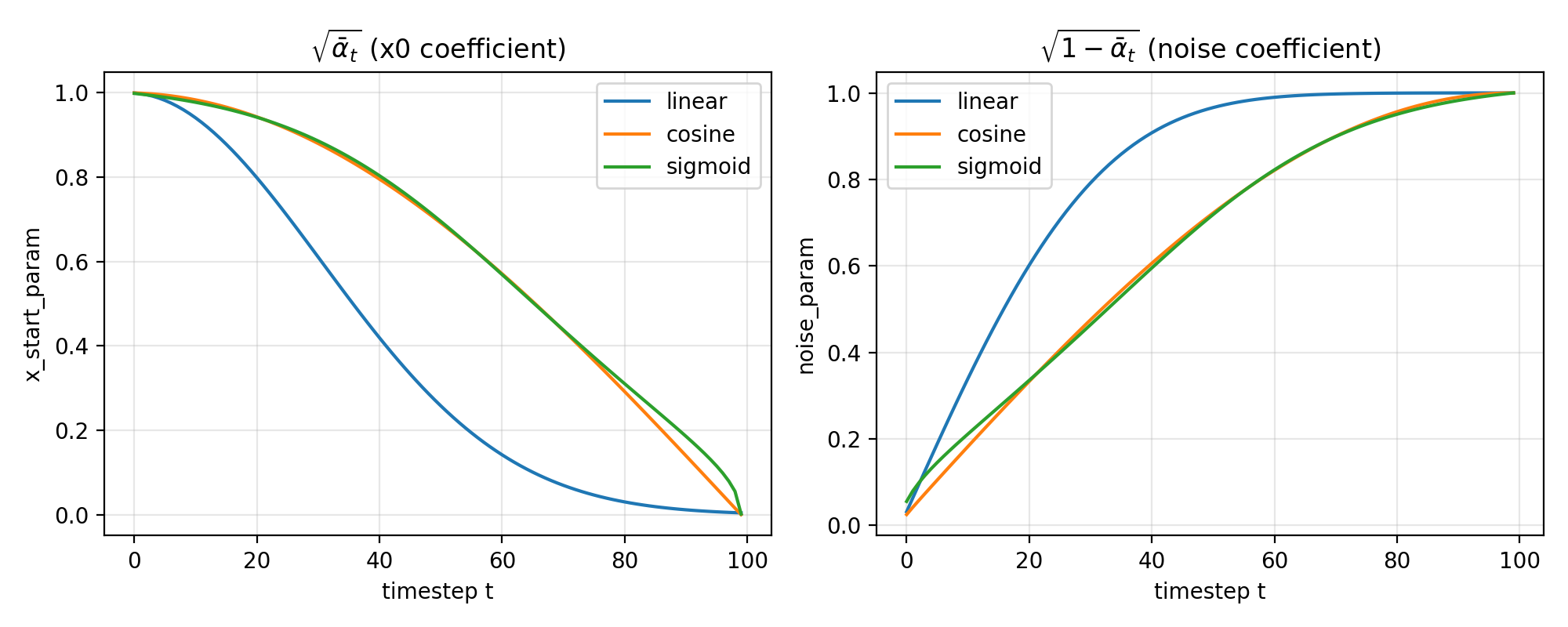
下面是可选的三种构建参数的方法: beta_schedule（“linear” | “cosine” | “sigmoid”）得到的 $\beta$ 以及 $\sqrt{{\bar{\alpha }}_t}$ & $\sqrt{1-{\bar{\alpha }}_t}$ ( $x_start_param $ & $noise_param $ )随时间步 t 变化的变化趋势。可以看出噪声的系数的变化率逐渐减小，说明噪声的扩散是逐渐减缓的。

Forward 文字过程表示

构建 context:

1. text_emb = text → CLIP tokenize&encoder

2. condition embedding = text_emb → drop → condition_mlp

   • condition_mlp = [affine(cond_d→context_d) → GELU → affine(context_d→context_d)];

3. time embedding = t → time_mlp

   • time_mlp = [SinusoidalPosEmb → affine(dim→context_d) → GELU → affine(context_d→context_d)];

4. context = condition embedding + time embedding

5. context = context → mlp → chunk & scale & shift

   • mlp = [GELU → Linear(context_dim → 2·dim_out)] ;

   • chunk & scale & shift: (scale, shift) = context.chunk(2, dim = 1); feature = feature * (scale + 1) + shift.

随后按顺序处理 UNet 结构以及 Up&Down Block 并传入 context。

UNet-forward()代码

    def forward(self, x, time, model_kwargs={}):"""Forward pass through the U-Net.Args:x: Input tensor of shape (batch_size, channels, height, width).time: Tensor of time steps of shape (batch_size,).model_kwargs: A dictionary of additional model inputs including"text_emb" (text embedding) of shape (batch_size, condition_dim).Returns:x: Output tensor of shape (batch_size, channels, height, width)."""if "cfg_scale" in model_kwargs:return self.cfg_forward(x, time, model_kwargs)# Embed time stepcontext = self.time_mlp(time)# Embed condition and add to contextcond_emb = model_kwargs["text_emb"]if cond_emb is None:cond_emb = torch.zeros(x.shape[0], self.condition_dim, device=x.device)if self.training:# Randomly drop conditionmask = (torch.rand(cond_emb.shape[0]) > self.uncond_prob).float()mask = mask[:, None].to(cond_emb.device)  # B x 1cond_emb = cond_emb * maskcontext = context + self.condition_mlp(cond_emb)# Initial convolutionx = self.init_conv(x)################################################################### TODO: Process `x` through the U-Net conditioned on the context.## 1. Downsampling:#    - Process `x` through each downsampling block with context.#    - After each ResNet block, save the output (feature maps) in a list or dict#      for use as skip connections in the upsampling path.#    - Make sure to pass the context to each ResNet block.## 2. Middle:#    - Process `x` through the middle blocks with context.## 3. Upsampling:#    - Process `x` through each upsampling block with context.#    - Before each ResNet block, concatenate the input with the corresponding#      skip connection from the downsampling path.#    - Make sure to pass the context to each ResNet block.##################################################################skips = []for res1, res2, down in self.downs:x = res1(x, context)skips.append(x)x = res2(x, context)skips.append(x)x = down(x)x = self.mid_block1(x, context)x = self.mid_block2(x, context)for up, res1, res2 in self.ups:x = up(x)x = torch.cat([x, skips.pop()], dim=1)x = res1(x, context)x = torch.cat([x, skips.pop()], dim=1)x = res2(x, context)################################################################### Final blockx = self.final_conv(x)return x

---

3. 损失 p_losses

第二个重要公式, 用于定义模型的损失:

$$x_t=\sqrt{{\bar{\alpha }}_t}{x}_0+\sqrt{1-{\bar{\alpha }}_t}\epsilon \text{\hspace{1em}(1)}$$

$$L_{\mathrm{simple}}(\theta ):={\mathbb{E}}_{t,{\mathbf{x}}_0,\mathbf{ϵ}}\left[{\Vert \mathbf{ϵ}-{\mathbf{ϵ}}_{\theta }(\sqrt{{\bar{\alpha }}_t}{\mathbf{x}}_0+\sqrt{1-{\bar{\alpha }}_t}\mathbf{ϵ},t)\Vert }^2\right]\text{\hspace{1em}(2)}$$

就是将取样+计算得到的 xt(t, x0, ε)和 context(text, t)传入模型，使输出值与原始噪声 ε 的差值最小，实现拟合效果。注意计算 loss 时需要乘 loss_weight 并取均值。

p_losses 代码如下：

    def p_losses(self, x_start, model_kwargs={}):b, nts = x_start.shape[0], self.num_timestepst = torch.randint(0, nts, (b,), device=x_start.device).long()  # (b,)x_start = self.normalize(x_start)  # (b, *)noise = torch.randn_like(x_start)  # (b, *)target = noise if self.objective == "pred_noise" else x_start  # (b, *)loss_weight = extract(self.loss_weight, t, target.shape)  # (b, *)loss = None##################################################################### TODO:# Implement the loss function according to Eq. (14) of the paper.# First, sample x_t from q(x_t | x_0) using the `q_sample` function.# Then, get model predictions by calling self.model with appropriate args.# Finally, compute the weighted MSE loss.# Approximately 3-4 lines of code.##################################################################### q_samplex_t = self.q_sample(x_start, t, noise)# modelpred = self.model(x_t, t, model_kwargs)# MSELossloss = ((pred - target) ** 2 * loss_weight).mean()####################################################################return loss

这样就构建好了损失函数。

4. p_sample

p_sample 实现的是从 xt -> x0 的去噪原理。是通过训练好的噪声预测模型得到噪声后计算分布，最终采样得到 $x_{t-1}$ 的过程。

第三个重要公式，描述的是由 xt&x0(or ε)得到 $x_{t-1}$ 的前向后验高斯分布。我们能够通过模型预测得到的 x0(ε)与从正态分布抽样得到的 xt 来对 $x_{t-1}$ 进行一个大致估计。这个公式在 q_posterior() 函数中实现。（T 足够大时分布近似为正态分布，因此任何一张标准正态分布采样得到的图片都是某个初始图片 x0 经过 T 个时间步之后得到的 xt）

$$\begin{array}{rlr}q({\mathbf{x}}_{t-1}|{\mathbf{x}}_t,{\mathbf{x}}_0)& =\mathcal{N}({\mathbf{x}}_{t-1};{\tilde{\mathbf{\mu }}}_t({\mathbf{x}}_t,{\mathbf{x}}_0),{\tilde{\beta }}_t\mathbf{I}),& (3)\\ \mathrm{where}{\bar{\mathbf{\mu }}}_t({\mathbf{x}}_t,{\mathbf{x}}_0)& :=\frac{\sqrt{{\bar{\alpha }}_{t-1}{\beta }_t}}{1-{\bar{\alpha }}_t}{\mathbf{x}}_0+\frac{\sqrt{{\alpha }_t}(1-{\bar{\alpha }}_{t-1})}{1-{\bar{\alpha }}_t}{\mathbf{x}}_t\mathrm{and}{\bar{\beta }}_t:=\frac{1-{\bar{\alpha }}_{t-1}}{1-{\bar{\alpha }}_t}{\beta }_t& \end{array}$$

注意计算过程中要对预测得到的 x0 进行裁剪使得其值范围在-1~1，避免计算后验均值时发散。

p_sample()代码如下:

    def p_sample(self, x_t, t: int, model_kwargs={}):"""Sample from p(x_{t-1} | x_t) according to Eq. (6) of the paper. Used only during inference.Args:x_t: (b, *) tensor. Noisy image.t: int. Sampling time step.model_kwargs: additional arguments for the model.Returns:x_tm1: (b, *) tensor. Sampled image."""t = torch.full((x_t.shape[0],), t, device=x_t.device, dtype=torch.long)  # (b,)x_tm1 = None  # sample x_{t-1} from p(x_{t-1} | x_t)################################################################### TODO: Implement the sampling step p(x_{t-1} | x_t) according to Eq. (6):## - Steps:#   1. Get the model prediction by calling self.model with appropriate args.#   2. The model output can be either noise or x_start depending on self.objective.#      You can recover the other by calling self.predict_start_from_noise or#      self.predict_noise_from_start as needed.#   3. Clamp predicted x_start to the valid range [-1, 1]. This ensures the#      generation remains stable during denoising iterations.#   4. Get the mean and std for q(x_{t-1} | x_t, x_0) using self.q_posterior,#      and sample x_{t-1}.################################################################### predict noise & calculate x_0pred = self.model(x_t, t, model_kwargs)if self.objective == "pred_noise":x0_hat = self.predict_start_from_noise(x_t, t, pred)else:x0_hat = pred# clampx0_hat = x0_hat.clamp(-1.0, 1.0)# mean & stdposterior_mean, posterior_std = self.q_posterior(x0_hat, x_t, t)# sample x_{t-1}noise = torch.zeros_like(x_t) if t[0] == 0 else torch.randn_like(x_t)x_tm1 = posterior_mean + posterior_std * noise##################################################################return x_tm1# 用到的q_posterior()def q_posterior(self, x_start, x_t, t):"""Get the posterior q(x_{t-1} | x_t, x_0) according to Eq. (6) and (7) of the paper.Args:x_start: (b, *) tensor. Predicted start image.x_t: (b, *) tensor. Noisy image.t: (b,) tensor. Time step.Returns:posterior_mean: (b, *) tensor. Mean of the posterior.posterior_std: (b, *) tensor. Std of the posterior."""posterior_mean = Noneposterior_std = None##################################################################### We have already implemented this method for you.c1 = extract(self.posterior_mean_coef1, t, x_t.shape)c2 = extract(self.posterior_mean_coef2, t, x_t.shape)posterior_mean = c1 * x_start + c2 * x_tposterior_std = extract(self.posterior_std, t, x_t.shape)####################################################################return posterior_mean, posterior_std

5. CFG(Classifier Free Guidance)

CFG 论文原文: https://arxiv.org/pdf/2207.12598

分类器自由引导（Classifier-Free Guidance, CFG）是在扩散模型推断阶段增强条件一致性的策略。模型在训练时以一定概率丢弃条件，从而同时学到有条件与无条件两种映射；在采样时对同一噪声状态分别走一次有条件与无条件前向，再将两者线性组合以放大与条件的一致性，同时尽量保持可采样性与稳定性。

给定噪声水平 λ 下的状态 $z_{\lambda }$ 与条件 c，设 ${\epsilon }_{\theta }(z_{\lambda },c)$ 为有条件的噪声预测，${\epsilon }_{\theta }(z_{\lambda })$ 为无条件（空条件）的噪声预测。引导后的噪声预测定义为

$${\widetilde{\mathbf{ϵ}}}_{\theta }({\mathbf{z}}_{\lambda },\mathbf{c})=(1+w){\mathbf{ϵ}}_{\theta }({\mathbf{z}}_{\lambda },\mathbf{c})-w{\mathbf{ϵ}}_{\theta }({\mathbf{z}}_{\lambda })\text{\hspace{1em}(4)}$$

其中 w ≥ 0 为引导强度。w = 0 时，退化为有条件预测；w 增大时，模型更强地朝向满足条件的方向更新，但多样性下降且可能出现过饱和或伪影。该式与更常见写法 $${ϵ}_{\theta }^{\text{guided}}={ϵ}_{\theta }(z_{\lambda })+s({ϵ}_{\theta }(z_{\lambda },c)-{ϵ}_{\theta }(z_{\lambda }))$$ 等价，只需令 s = 1 + w。实际实现中对同一 $z_{\lambda }$ 计算两次前向，得到 ${\epsilon }_{\theta }(z_{\lambda },c)$ 与 ${\epsilon }_{\theta }(z_{\lambda })$，按上式组合得到总预测噪声 ${\widetilde{\mathbf{ϵ}}}_{\theta }$，再用于一步去噪更新。

cfg_forward()代码如下:

def cfg_forward(self, x, time, model_kwargs={}):"""Classifier-free guidance forward pass. model_kwargs should contain `cfg_scale`."""cfg_scale = model_kwargs.pop("cfg_scale")print("Classifier-free guidance scale:", cfg_scale)model_kwargs = copy.deepcopy(model_kwargs)################################################################### TODO: Apply classifier-free guidance using Eq. (6) from# https://arxiv.org/pdf/2207.12598 i.e.# x = (scale + 1) * eps(x_t, cond) - scale * eps(x_t, empty)## You will have to call self.forward two times.# For unconditional sampling, pass None in`text_emb`.################################################################### Conditional predictioncond_out = self.forward(x, time, model_kwargs)# Unconditional prediction (drop condition)uncond_kwargs = copy.deepcopy(model_kwargs)uncond_kwargs["text_emb"] = Noneuncond_out = self.forward(x, time, uncond_kwargs)# Classifier-free guidance combinationx = (cfg_scale + 1.0) * cond_out - cfg_scale * uncond_out##################################################################return x

6. Train & Sample

训练阶段以随机时刻的加噪样本为监督信号。给定干净样本 x0，先采样 ϵ∼N(0, I) 并构造 $$x_t=\sqrt{{\bar{\alpha }}_t},x_0+\sqrt{1-{\bar{\alpha }}_t},ϵ,{\alpha }_t=1-{\beta }_t,{\bar{\alpha }}_t=\prod _{s=1}^t{\alpha }_s$$（公式 1） 。将 (xt, t) 与可选条件 c 输入网络 ${ϵ}_{\theta }(x_t,t,c)$，最小化去噪损失 $$\mathbb{E}\ast t,x_0,ϵ[|ϵ-{ϵ}_{\theta }(x_t,t,c){|}^2]$$ （公式 2）。模型据此学会在任意噪声级别下的去噪方向。实践中对 t 进行均匀采样，对图像做归一化，并用时间嵌入编码 t。

一些关键点会影响稳定性与质量。噪声日程 (βt) 与 α¯t 的设定至关重要，常用线性或余弦日程。目标参数化影响优化难度：预测 ϵ 最常见，也可预测 x0 或 v。方差通常固定为论文中的形式（如 β~t），也有可学习方差的变体。条件建模可在训练时随机丢弃条件以支持分类器自由引导，在推断时通过引导强度 w 调节条件一致性。工程层面常配合权重 EMA、梯度裁剪与混合精度训练，并注意与归一化、数据增广的兼容。

采样阶段从 xT∼N(0, I) 出发，按学习到的逆向过程逐步得到 xt−1。在固定方差设定下，给定网络的噪声预测可写出均值 $${\mu }_{\theta }(x_t,t)=\frac{1}{\sqrt{{\alpha }_t}}!\left(x_t-\frac{1-{\alpha }_t}{\sqrt{1-{\bar{\alpha }}_t}},{ϵ}_{\theta }(x_t,t,c)\right)$$（公式 3），再以 $$x_{t-1}={\mu }_{\theta }(x_t,t)+{\sigma }_{t}z,z\sim \mathcal{N}(0,I)$$ 递推至 t = 0。该过程本质是在已学习的概率模型中进行逐步抽样，而非一次性的确定性生成，因此更准确的描述为采样 Sample。

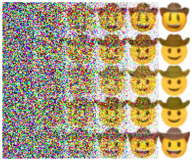
完全保留条件的采样：

使用 CFG，引导强度 w 为 0.5 的采样：

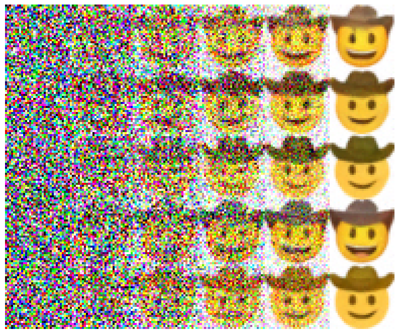
在此次采样过程中没有太大差别。可能因为加强幅度较小效果不明显，在此不做深入研究。

相关概念

概念	解释
SinusoidalPosEmb	SinusoidalPosEmb 是将标量时间步 t 映射为高维向量的固定（不学习）正弦–余弦特征。它与 Transformer 中的 sinusoidal positional encoding 同源，只是核心参数从“序列位置”换成“扩散过程中的时间位置”。
时间步 t 和噪声 ε 的采样	t 的采样：训练时从离散区间 [0, T-1] 里做“均匀随机”采样（不是正态），保证模型在所有噪声强度上都能学会去噪。 噪声 ε 的采样：从标准正态分布 N(0, I) 采样，用于前向扩散 q(x_t|x_0) 和训练目标（若预测噪声）。

函数	作用
nn.Upsample(scale_factor = 2, mode = “bilinear”)	把特征图在空间维度上放大 2 倍，使用双线性插值；不改变通道数、无可学习参数。
context.chunk(2, dim = 1)	context（如时间步、文本或类别嵌入）被映射为每个通道的一对参数，分别控制“放大/缩小”和“偏移”。实现时按通道维对半切分为两块得到 scale 与 shift，各为 (B, dim_out, 1, 1)。
torch.cumprod(alphas, dim = 0)	每个位置的值为该位置及前面所有位置数值的乘积