无监督机器学习算法案例(Python)
Kmeans算法
聚类算法,目标是将数据集划分为 K 个预定义的不相交的簇(cluster),使得每个数据点都属于离它最近的簇的中心(称为“质心”)所代表的簇。
核心思想:物以类聚。通过迭代计算,不断更新簇的质心位置,最终使得簇内的点尽可能相似(距离小),簇间的点尽可能不同。
- 实现2D数据自动聚类,预测V1=80,v2=60的数据类别
- 计算预测准确率,完整结果矫正
- 采用KNN、Means算法,重复步骤1-2
import pandas as pd
import numpy as np
data = pd.read_csv('data.csv')
data.head()

X = data.drop(['labels'],axis=1)
y = data.loc[:,'labels']pd.value_counts(y)%matplotlib inline
from matplotlib import pyplot as plt
fig1 = plt.figure()
plt.scatter(X.log[:,'V1'],X.loc[:,'V2'])
plt.title("un-labled data")
plt.xlabel('V1')
plt.ylabel('V2')
plt.show()
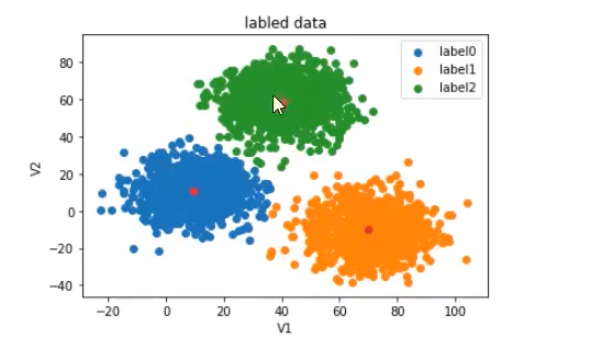
fig1 = plt.figure()
#在二维平面上,用散点图绘制所有类别标签为 0 的样本,其中 x 坐标是 V1 特征的值,y 坐标是 V2 特征的值。
label0 = plt.scatter(X.loc[:,'V1'][y==0],X.loc[:,'V2'][y==0])
label1 = plt.scatter(X.loc[:,'V1'][y==1],X.loc[:,'V2'][y==1])
label2 = plt.scatter(X.loc[:,'V1'][y==2],X.loc[:,'V2'][y==2])plt.title("labled data")
plt.xlabel('V1')
plt.ylabel('V2')
plt.legend((label0,label1,label2),('label0','label1','label2'))
plt.show()

print(X.shape,y.shape)from sklearn.cluster import KMeans
KM = KMeans(n_clusters=3,random_state=0)
KM.fit(X)#训练好模型,找出中心点
centers = KM.cluster_centers_
fig3 = plt.figure()
label0 = plt.scatter(X.loc[:,'V1'][y==0],X.loc[:,'V2'][y==0])
label1 = plt.scatter(X.loc[:,'V1'][y==1],X.loc[:,'V2'][y==1])
label2 = plt.scatter(X.loc[:,'V1'][y==2],X.loc[:,'V2'][y==2])plt.title("labled data")
plt.xlabel('V1')
plt.ylabel('V2')
plt.legend((label0,label1,label2),('label0','label1','label2'))
plt.scatter(centers[:,0],centers[:,1])
plt.show()
#测试
y_predict_test = KM.predict([[80,60]])
print(y_predict_test)y_predict = KM.predict(X)
print(pd.value_counts(y_predict),pd.value_counts(y))
from sklearn.metrics import accuracy_score
accuracy = accuracy_score(y,y_predict)
print(accuracy)
电商客户细分
import numpy as np
import pandas as pd
from sklearn.cluster import KMeans
from sklearn.preprocessing import StandardScaler
from sklearn.metrics import silhouette_score
import matplotlib.pyplot as plt
import seaborn as sns
from sklearn.datasets import make_blobs# 企业级设置
plt.style.use('seaborn-v0_8')
np.random.seed(42)class CustomerSegmentation:def __init__(self):self.scaler = StandardScaler()self.model = Nonedef generate_enterprise_data(self, n_samples=1000):"""生成模拟的企业级客户数据"""# 创建具有明显集群结构的数据centers = [[30000, 2000], [80000, 8000], [120000, 15000], [50000, 3000]]X, _ = make_blobs(n_samples=n_samples, centers=centers, cluster_std=[5000, 8000, 10000, 4000], random_state=42)# 添加一些噪声和异常值X = np.vstack([X, np.random.uniform(20000, 150000, (50, 2))])# 创建DataFramedf = pd.DataFrame(X, columns=['Annual_Income', 'Annual_Spending'])# 确保数据合理性df['Annual_Income'] = np.abs(df['Annual_Income'])df['Annual_Spending'] = np.abs(df['Annual_Spending'])return dfdef preprocess_data(self, df):"""数据预处理"""# 处理异常值 - 使用IQR方法Q1 = df.quantile(0.25)Q3 = df.quantile(0.75)IQR = Q3 - Q1df = df[~((df < (Q1 - 1.5 * IQR)) | (df > (Q3 + 1.5 * IQR))).any(axis=1)]# 数据标准化scaled_data = self.scaler.fit_transform(df)return scaled_data, df.indexdef find_optimal_k(self, data, max_k=10):"""使用肘部法则和轮廓系数确定最佳K值"""wcss = []  # 簇内平方和silhouette_scores = []k_range = range(2, max_k + 1)for k in k_range:kmeans = KMeans(n_clusters=k, init='k-means++', random_state=42, n_init=10)kmeans.fit(data)wcss.append(kmeans.inertia_)if k > 1:  # 轮廓系数需要至少2个簇score = silhouette_score(data, kmeans.labels_)silhouette_scores.append(score)# 绘制肘部法则图plt.figure(figsize=(15, 5))plt.subplot(1, 2, 1)plt.plot(k_range, wcss, 'bo-')plt.xlabel('Number of Clusters (K)')plt.ylabel('Within-Cluster Sum of Square (WCSS)')plt.title('Elbow Method for Optimal K')plt.subplot(1, 2, 2)plt.plot(range(2, max_k + 1), silhouette_scores, 'ro-')plt.xlabel('Number of Clusters (K)')plt.ylabel('Silhouette Score')plt.title('Silhouette Score for Different K Values')plt.tight_layout()plt.show()return k_range, wcss, silhouette_scoresdef train_model(self, data, n_clusters=4):"""训练K-Means模型"""self.model = KMeans(n_clusters=n_clusters, init='k-means++', random_state=42, n_init=10)clusters = self.model.fit_predict(data)return clustersdef analyze_clusters(self, original_df, clusters):"""分析聚类结果"""df_with_clusters = original_df.copy()df_with_clusters['Cluster'] = clusters# 计算每个簇的统计信息cluster_stats = df_with_clusters.groupby('Cluster').agg({'Annual_Income': ['count', 'mean', 'std', 'min', 'max'],'Annual_Spending': ['mean', 'std', 'min', 'max']}).round(2)print("=== 客户分群统计 ===")print(cluster_stats)return df_with_clustersdef visualize_results(self, original_df, clusters):"""可视化聚类结果"""plt.figure(figsize=(12, 5))# 原始数据plt.subplot(1, 2, 1)plt.scatter(original_df['Annual_Income'], original_df['Annual_Spending'], alpha=0.6, s=30)plt.xlabel('Annual Income ($)')plt.ylabel('Annual Spending ($)')plt.title('Original Customer Data')# 聚类结果plt.subplot(1, 2, 2)scatter = plt.scatter(original_df['Annual_Income'], original_df['Annual_Spending'], c=clusters, cmap='viridis', alpha=0.7, s=40)plt.xlabel('Annual Income ($)')plt.ylabel('Annual Spending ($)')plt.title('Customer Segmentation with K-Means')plt.colorbar(scatter, label='Cluster')plt.tight_layout()plt.show()def get_cluster_profiles(self, df_with_clusters):"""生成客户群画像"""profiles = {}for cluster_id in df_with_clusters['Cluster'].unique():cluster_data = df_with_clusters[df_with_clusters['Cluster'] == cluster_id]profile = {'size': len(cluster_data),'avg_income': cluster_data['Annual_Income'].mean(),'avg_spending': cluster_data['Annual_Spending'].mean(),'spending_ratio': (cluster_data['Annual_Spending'] / cluster_data['Annual_Income']).mean() * 100}# 根据特征定义客户类型if profile['avg_income'] > 80000 and profile['avg_spending'] > 10000:profile['type'] = '高价值客户'elif profile['avg_income'] > 80000 and profile['avg_spending'] <= 10000:profile['type'] = '潜力客户'elif profile['avg_income'] <= 80000 and profile['spending_ratio'] > 15:profile['type'] = '精明消费者'else:profile['type'] = '普通客户'profiles[cluster_id] = profilereturn profiles# 企业级应用示例
def run_customer_segmentation():print("🚀 开始电商客户细分项目...")# 初始化segmentation = CustomerSegmentation()# 1. 生成企业数据print("📊 生成模拟客户数据...")customer_data = segmentation.generate_enterprise_data(1000)print(f"生成数据形状: {customer_data.shape}")# 2. 数据预处理print("🔧 数据预处理中...")processed_data, valid_indices = segmentation.preprocess_data(customer_data)valid_data = customer_data.loc[valid_indices]print(f"预处理后数据形状: {processed_data.shape}")# 3. 寻找最佳K值print("📈 寻找最佳聚类数量...")k_range, wcss, silhouette_scores = segmentation.find_optimal_k(processed_data, max_k=8)# 基于轮廓系数选择最佳Koptimal_k = np.argmax(silhouette_scores) + 2  # +2 因为从K=2开始print(f"推荐聚类数量: {optimal_k}")# 4. 训练模型print("🤖 训练K-Means模型中...")clusters = segmentation.train_model(processed_data, n_clusters=optimal_k)# 5. 分析结果print("📋 分析聚类结果...")df_with_clusters = segmentation.analyze_clusters(valid_data, clusters)# 6. 可视化print("🎨 生成可视化结果...")segmentation.visualize_results(valid_data, clusters)# 7. 生成客户画像print("👥 创建客户群画像...")profiles = segmentation.get_cluster_profiles(df_with_clusters)for cluster_id, profile in profiles.items():print(f"\n集群 {cluster_id} ({profile['type']}):")print(f"  客户数量: {profile['size']}")print(f"  平均年收入: ${profile['avg_income']:,.0f}")print(f"  平均年消费: ${profile['avg_spending']:,.0f}")print(f"  消费收入比: {profile['spending_ratio']:.1f}%")return segmentation, df_with_clusters, profiles# 运行项目
if __name__ == "__main__":model, results, profiles = run_customer_segmentation()
Mean-shift算法
与 K-Means 需要预先指定 K 不同,Mean-Shift 不需要指定簇的数量,它可以自动发现数据中的模式并确定簇的个数。
核心思想:想象特征空间是一个密度场。算法从每个数据点出发,朝着密度增加的方向(即点最密集的区域)不断移动,直到收敛。所有最终收敛到同一点的原始点被归为同一个簇。这个收敛点就是模式的中心(峰值)。
工作原理:
- 算法会围绕每个数据点画一个半径为 带宽(bandwidth) 的圆(或超球体)。
- 计算圆内所有点的均值,将圆心移动到这个均值点。
- 重复步骤 2,直到圆心的移动非常小(收敛)。这个收敛的区域就是一个簇的质心。
- 多个起点收敛到同一个质心的被合并为一个簇。
from sklearn.cluster import MeanShift,estimate_bandwidth
bw = estimate_bandwidth(X,n_samples=500)
print(bw)ms = MeanShift(bandwidth=bw)
ms.fit(X)y_predict_ms = ms.predict(X)
print(pd.value_counts(y_predict_ms))
网络安全异常检测
import numpy as np
import pandas as pd
from sklearn.cluster import MeanShift, estimate_bandwidth
from sklearn.preprocessing import StandardScaler, RobustScaler
from sklearn.metrics import silhouette_score, calinski_harabasz_score
from sklearn.datasets import make_blobs
import matplotlib.pyplot as plt
import seaborn as sns
from mpl_toolkits.mplot3d import Axes3D
from sklearn.decomposition import PCAclass NetworkSecurityMonitor:def __init__(self):self.scaler = RobustScaler()  # 使用RobustScaler处理异常值self.model = Nonedef generate_network_data(self, n_samples=2000):"""生成模拟的网络流量数据"""# 创建正常流量集群normal_centers = [[100, 50, 10, 5, 1000],    # 正常网页浏览[500, 200, 30, 15, 5000],   # 文件下载[50, 20, 5, 2, 200]         # API调用]# 创建异常流量(攻击)anomaly_centers = [[5000, 3000, 500, 100, 10],  # DDoS攻击[10, 1000, 2, 500, 5],       # 端口扫描[1000, 50, 200, 5, 10000]    # 数据泄露]# 生成正常数据(95%)X_normal, _ = make_blobs(n_samples=int(n_samples * 0.95),centers=normal_centers,cluster_std=[20, 50, 10],random_state=42)# 生成异常数据(5%)X_anomaly, _ = make_blobs(n_samples=int(n_samples * 0.05),centers=anomaly_centers,cluster_std=[100, 50, 200],random_state=42)# 合并数据X = np.vstack([X_normal, X_anomaly])y = np.array([0] * len(X_normal) + [1] * len(X_anomaly))# 创建DataFramefeature_names = ['Packet_Count', 'Connection_Count', 'Error_Rate', 'Port_Activity', 'Data_Volume']df = pd.DataFrame(X, columns=feature_names)df['Is_Anomaly'] = y# 添加一些随机噪声noise = np.random.normal(0, 10, (n_samples, 5))df[feature_names] += noise# 确保正值df[feature_names] = np.abs(df[feature_names])return dfdef preprocess_data(self, df):"""数据预处理"""features = df.drop('Is_Anomaly', axis=1)# 使用RobustScaler处理异常值scaled_features = self.scaler.fit_transform(features)return scaled_features, df['Is_Anomaly']def estimate_optimal_bandwidth(self, data, quantile=0.2):"""估计最佳带宽参数"""bandwidth = estimate_bandwidth(data, quantile=quantile, n_samples=500)print(f"估计的带宽: {bandwidth:.4f}")return bandwidthdef train_mean_shift(self, data, bandwidth=None):"""训练Mean-Shift模型"""if bandwidth is None:bandwidth = self.estimate_optimal_bandwidth(data)self.model = MeanShift(bandwidth=bandwidth, bin_seeding=True, n_jobs=-1)clusters = self.model.fit_predict(data)print(f"发现的集群数量: {len(np.unique(clusters))}")return clustersdef analyze_clusters(self, data, clusters, true_labels):"""分析聚类结果"""results = pd.DataFrame({'Cluster': clusters,'Is_Anomaly': true_labels})# 计算每个集群的异常比例cluster_stats = results.groupby('Cluster').agg({'Is_Anomaly': ['count', 'mean', 'sum']}).round(4)cluster_stats.columns = ['Total_Count', 'Anomaly_Ratio', 'Anomaly_Count']cluster_stats = cluster_stats.sort_values('Anomaly_Ratio', ascending=False)print("=== 集群异常分析 ===")print(cluster_stats)# 识别异常集群anomaly_clusters = cluster_stats[cluster_stats['Anomaly_Ratio'] > 0.7].index.tolist()print(f"识别出的异常集群: {anomaly_clusters}")return results, anomaly_clustersdef evaluate_detection(self, true_labels, clusters, anomaly_clusters):"""评估异常检测性能"""# 将属于异常集群的点标记为预测异常predicted_anomalies = np.isin(clusters, anomaly_clusters).astype(int)from sklearn.metrics import classification_report, confusion_matrixprint("=== 异常检测性能 ===")print(classification_report(true_labels, predicted_anomalies, target_names=['正常', '异常']))# 混淆矩阵plt.figure(figsize=(10, 4))cm = confusion_matrix(true_labels, predicted_anomalies)sns.heatmap(cm, annot=True, fmt='d', cmap='Reds',xticklabels=['正常', '异常'], yticklabels=['正常', '异常'])plt.ylabel('真实标签')plt.xlabel('预测标签')plt.title('异常检测混淆矩阵')plt.show()return predicted_anomaliesdef visualize_results(self, data, clusters, true_labels, predicted_anomalies):"""可视化结果"""# 使用PCA进行降维以便可视化pca = PCA(n_components=2)data_2d = pca.fit_transform(data)plt.figure(figsize=(18, 6))# 真实标签plt.subplot(1, 3, 1)scatter = plt.scatter(data_2d[:, 0], data_2d[:, 1], c=true_labels, cmap='coolwarm', alpha=0.7)plt.colorbar(scatter, label='真实标签 (0=正常, 1=异常)')plt.title('真实网络流量分布')plt.xlabel('PCA Component 1')plt.ylabel('PCA Component 2')# 聚类结果plt.subplot(1, 3, 2)scatter = plt.scatter(data_2d[:, 0], data_2d[:, 1], c=clusters, cmap='viridis', alpha=0.7)plt.colorbar(scatter, label='集群')plt.title('Mean-Shift 聚类结果')plt.xlabel('PCA Component 1')plt.ylabel('PCA Component 2')# 预测结果plt.subplot(1, 3, 3)colors = ['blue' if x == 0 else 'red' for x in predicted_anomalies]plt.scatter(data_2d[:, 0], data_2d[:, 1], c=colors, alpha=0.7)plt.title('预测的异常点 (红色=异常)')plt.xlabel('PCA Component 1')plt.ylabel('PCA Component 2')plt.tight_layout()plt.show()# 3D可视化(可选)if data.shape[1] >= 3:fig = plt.figure(figsize=(12, 8))ax = fig.add_subplot(111, projection='3d')pca_3d = PCA(n_components=3)data_3d = pca_3d.fit_transform(data)scatter = ax.scatter(data_3d[:, 0], data_3d[:, 1], data_3d[:, 2],c=predicted_anomalies, cmap='coolwarm', alpha=0.6)ax.set_xlabel('PCA Component 1')ax.set_ylabel('PCA Component 2')ax.set_zlabel('PCA Component 3')plt.colorbar(scatter, label='预测标签 (0=正常, 1=异常)')plt.title('3D网络流量异常检测')plt.show()def feature_analysis(self, original_df, clusters):"""特征分析"""df_analysis = original_df.copy()df_analysis['Cluster'] = clusters# 分析每个集群的特征统计cluster_features = df_analysis.groupby('Cluster').mean()plt.figure(figsize=(15, 10))sns.heatmap(cluster_features, annot=True, cmap='YlOrRd', fmt='.1f')plt.title('各集群特征均值热力图')plt.show()return cluster_features# 企业级应用示例
def run_network_security():print("🚀 开始网络安全异常检测项目...")# 初始化security_monitor = NetworkSecurityMonitor()# 1. 生成网络数据print("📊 生成模拟网络流量数据...")network_data = security_monitor.generate_network_data(2000)print(f"异常流量比例: {network_data['Is_Anomaly'].mean():.3f}")# 2. 数据预处理print("🔧 数据预处理中...")scaled_data, true_labels = security_monitor.preprocess_data(network_data)# 3. 训练Mean-Shift模型print("🤖 训练Mean-Shift模型中...")clusters = security_monitor.train_mean_shift(scaled_data, quantile=0.15)# 4. 分析集群print("📋 分析聚类结果...")results, anomaly_clusters = security_monitor.analyze_clusters(scaled_data, clusters, true_labels)# 5. 评估检测性能print("📊 评估异常检测性能...")predicted_anomalies = security_monitor.evaluate_detection(true_labels, clusters, anomaly_clusters)# 6. 可视化结果print("🎨 生成可视化结果...")security_monitor.visualize_results(scaled_data, clusters, true_labels, predicted_anomalies)# 7. 特征分析print("📈 进行特征分析...")cluster_features = security_monitor.feature_analysis(network_data.drop('Is_Anomaly', axis=1), clusters)print("\n=== 异常集群特征分析 ===")for cluster_id in anomaly_clusters:print(f"\n异常集群 {cluster_id} 的特征均值:")print(cluster_features.loc[cluster_id])return security_monitor, network_data, results# 运行项目
if __name__ == "__main__":monitor, data, results = run_network_security()