朴素贝叶斯分类器

​​多项式朴素贝叶斯

适用场景：​​ 离散型特征数据（特别是文本数据）。

典型应用：​​ 文本分类（如统计单词出现次数）。

导入方式：​​ from sklearn.naive_bayes import MultinomialNB。

高斯朴素贝叶斯

适用场景：​​ 连续型特征数据（具体数值，符合或近似正态分布）。

​​典型应用：​​ 处理连续变量（如测量值）。

​​导入方式：​​ from sklearn.naive_bayes import GaussianNB

伯努利朴素贝叶斯

适用场景：​​ 离散型特征数据且取值​​只有两种​​（0/1, True/False）。

典型应用：​​ 文本分类（侧重特征是否出现，而非出现次数）。​​

导入方式：​​ from sklearn.naive_bayes import BernoulliNB

模型选择取决于特征类型：​​

文本/离散计数 -- MultinomialNB

连续数值 --GaussianNB

二值特征 -- BernoulliNB

多项式模型不适合处理连续变量，高斯模型不适合处理离散变量。

应用

import numpy as np
import matplotlib.pyplot as plt
from sklearn.datasets import load_digits
from sklearn.model_selection import train_test_split
from sklearn.naive_bayes import GaussianNB, MultinomialNB, BernoulliNB
from sklearn.metrics import accuracy_score, confusion_matrix, ConfusionMatrixDisplay
from sklearn.preprocessing import MinMaxScaler
# 设置中文显示
plt.rcParams["font.family"] = ["SimHei", "Microsoft YaHei", "SimSun"]
plt.rcParams['axes.unicode_minus'] = False

# 1. 加载手写数字数据集
digits = load_digits()
print(f"数据集包含 {len(digits.images)} 个手写数字样本")
print(f"每个数字是 {digits.images[0].shape[0]}x{digits.images[0].shape[1]} 像素的图像")

# 2. 数据预处理
# 将图像数据展平为特征向量
X = digits.images.reshape((len(digits.images), -1))#将8x8图像展平为64维特征向量
y = digits.target
print("特征值:",X)
print("标签",y)

# 将像素值归一化到[0, 1]范围
scaler = MinMaxScaler()
X = scaler.fit_transform(X)
# 3. 划分训练集和测试集
X_train, X_test, y_train, y_test = train_test_split(X, y, test_size=0.3, random_state=42
)
print(f"\n训练样本数: {X_train.shape[0]} | 测试样本数: {X_test.shape[0]}")
# 4. 创建并训练朴素贝叶斯模型
# 尝试三种不同的朴素贝叶斯变体
models = {"高斯朴素贝叶斯": GaussianNB(),"多项式朴素贝叶斯": MultinomialNB(),"伯努利朴素贝叶斯": BernoulliNB(binarize=0.5)  # 二值化阈值设为0.5
}# 存储结果
results = {}# 训练并评估每个模型
for name, model in models.items():print(f"\n训练 {name} 模型...")model.fit(X_train, y_train)# 在测试集上预测y_pred = model.predict(X_test)# 计算准确率accuracy = accuracy_score(y_test, y_pred)results[name] = accuracyprint(f"{name} 准确率: {accuracy:.4f}")

# 5. 可视化模型比较
# 绘制准确率比较图
plt.figure(figsize=(10, 6))
plt.bar(results.keys(), results.values(), color=['yellow', 'green', 'red'])
plt.title('不同朴素贝叶斯模型准确率比较')
plt.ylabel('准确率')
plt.ylim(0.7, 0.9)
plt.grid(axis='y', alpha=0.3)# 在柱子上方添加准确率数值
for i, v in enumerate(results.values()):plt.text(i, v + 0.005, f"{v:.4f}", ha='center', fontsize=10)plt.show()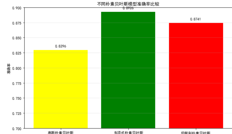

# 6. 使用最佳模型进行详细分析
# 选择准确率最高的模型
best_model_name = max(results, key=results.get)#遍历字典的所有值（准确率）
best_model = models[best_model_name]
print(f"\n最佳模型: {best_model_name} (准确率: {results[best_model_name]:.4f})")# 在测试集上评估最佳模型
y_pred = best_model.predict(X_test)# 显示混淆矩阵
cm = confusion_matrix(y_test, y_pred)#计算混淆矩阵
disp = ConfusionMatrixDisplay(confusion_matrix=cm, display_labels=digits.target_names)#设置标签为0-9
disp.plot(cmap='Blues')
plt.title(f'{best_model_name} 混淆矩阵')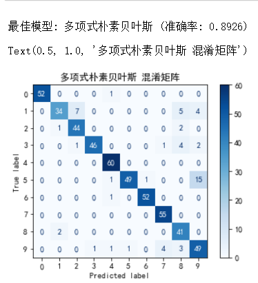

# 7. 可视化一些预测结果
# 随机选择一些测试样本进行可视化
n_samples = 10
indices = np.random.choice(range(len(X_test)), n_samples, replace=False)#生成测试集所有样本的索引plt.figure(figsize=(15, 6))
for i, idx in enumerate(indices):# 原始图像ax = plt.subplot(2, n_samples, i + 1)plt.imshow(X_test[idx].reshape(8, 8), cmap=plt.cm.gray_r, interpolation='nearest')#禁用平滑，保留像素感plt.title(f"真实: {y_test[idx]}\n预测: {y_pred[idx]}")plt.axis('off')# 模型预测概率if hasattr(best_model, 'predict_proba'):#检查模型是否支持概率预测probs = best_model.predict_proba(X_test[idx].reshape(1, -1))[0]#获取每个类别的预测概率ax = plt.subplot(2, n_samples, i + n_samples + 1)plt.bar(range(10), probs, color='skyblue')plt.title('预测概率')plt.xlabel('数字')plt.ylabel('概率')plt.ylim(0, 1)plt.xticks(range(10))plt.tight_layout()#自动调整子图间距
plt.show()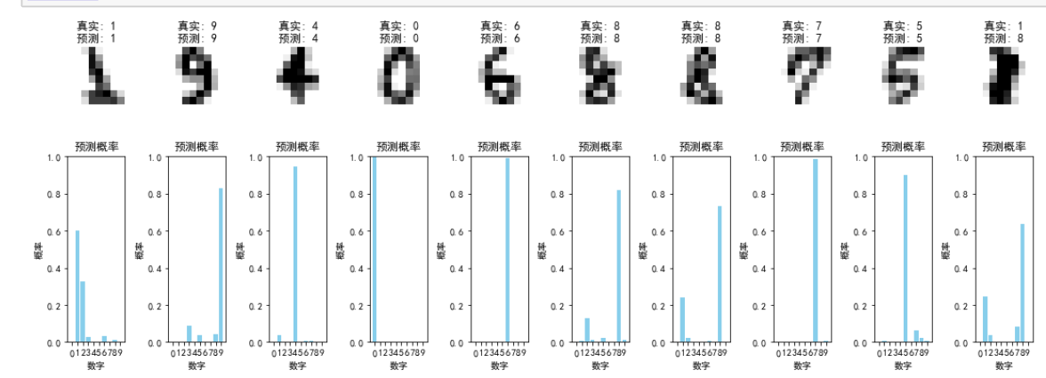

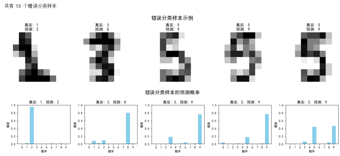
# 8. 分析错误分类的样本
# 找出预测错误的样本
errors = np.where(y_pred != y_test)[0]#创建布尔数组（True表示预测错误）
print(f"\n共有 {len(errors)} 个错误分类样本")if len(errors) > 0:# 随机选择一些错误样本进行可视化n_errors = min(5, len(errors))error_indices = np.random.choice(errors, n_errors, replace=False)plt.figure(figsize=(15, 3))for i, idx in enumerate(error_indices):ax = plt.subplot(1, n_errors, i + 1)plt.imshow(X_test[idx].reshape(8, 8), cmap=plt.cm.gray_r, interpolation='nearest')plt.title(f"真实: {y_test[idx]}\n预测: {y_pred[idx]}")plt.axis('off')plt.suptitle('错误分类样本示例', fontsize=16)plt.tight_layout()plt.show()# 分析错误样本的预测概率if hasattr(best_model, 'predict_proba'):#返回每个类别的预测概率plt.figure(figsize=(15, 3))for i, idx in enumerate(error_indices):probs = best_model.predict_proba(X_test[idx].reshape(1, -1))[0]ax = plt.subplot(1, n_errors, i + 1)plt.bar(range(10), probs, color='skyblue')plt.title(f"真实: {y_test[idx]}, 预测: {y_pred[idx]}")plt.xlabel('数字')plt.ylabel('概率')plt.ylim(0, 1)plt.xticks(range(10))plt.suptitle('错误分类样本的预测概率', fontsize=16)plt.tight_layout()plt.show()