机器学习(3)---线性算法,决策树,神经网络,支持向量机
1、概述
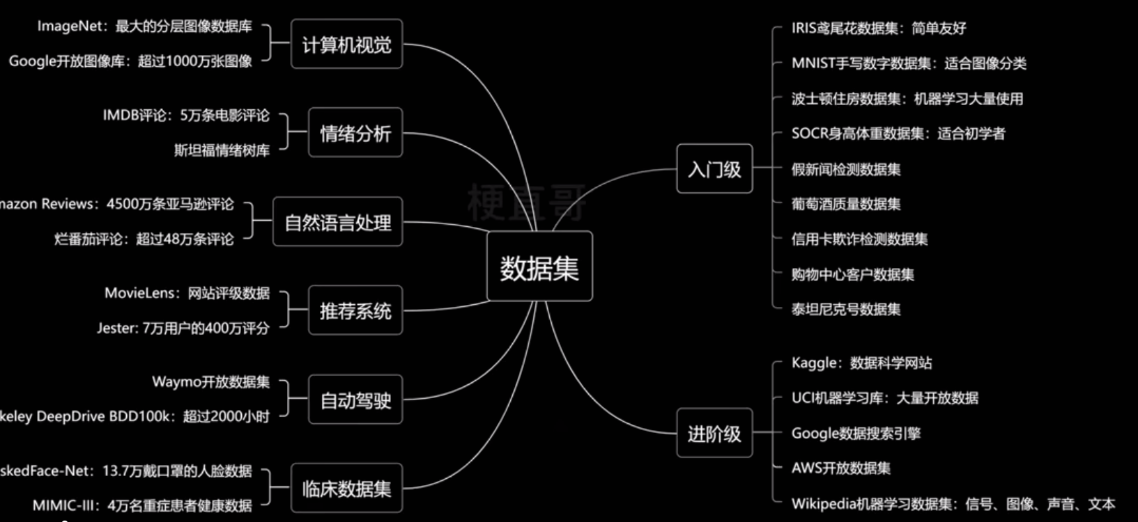
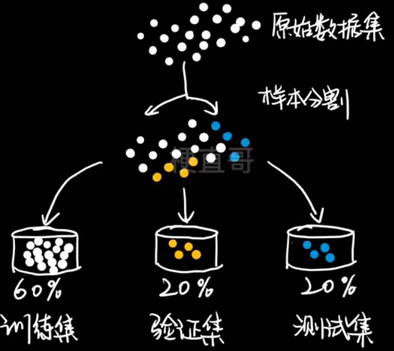
- 数据集
最常用的公开数据集
- 数据集 dataset
- 样本 sample
- 特征 feature
- 类别标记 label
- 向量 vector
- 矩阵 matrix
- 机器学习的任务
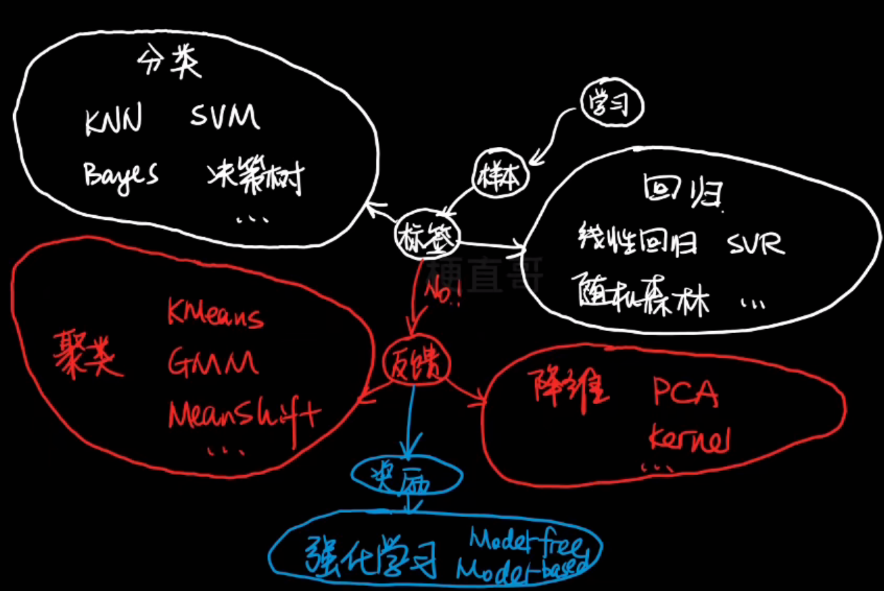
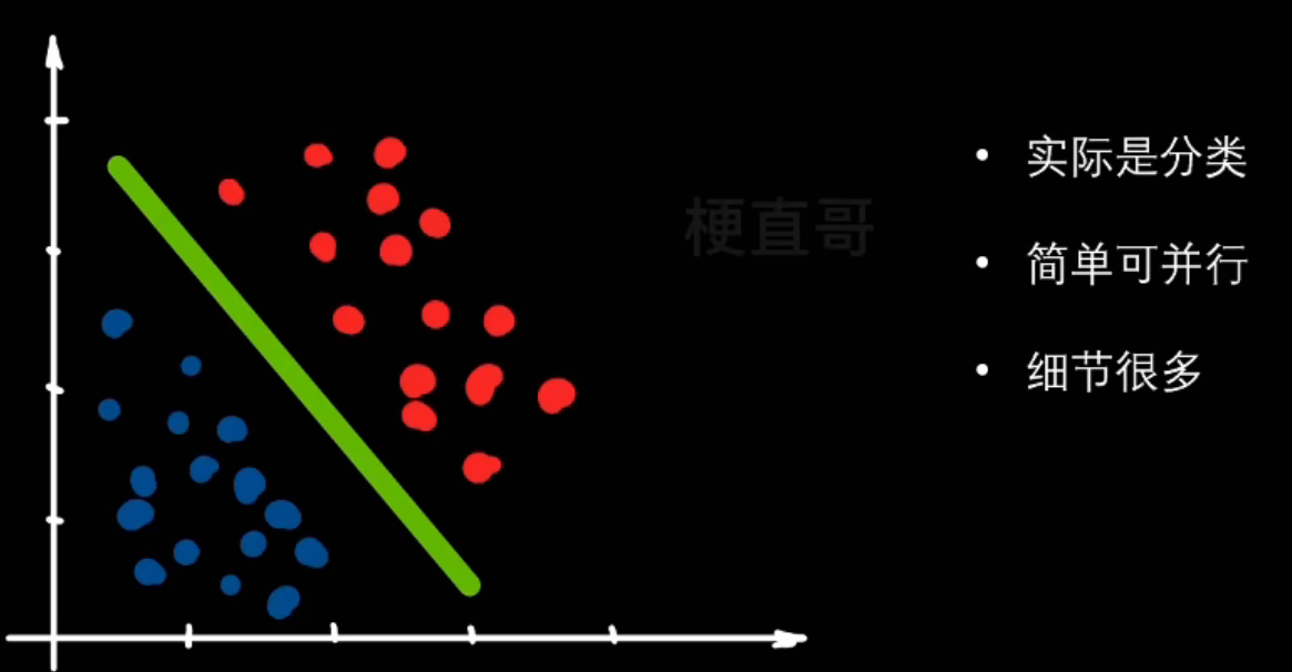
- 分类任务:已知样本特征,判断样本类别。常见有二分类,多分类,多标签分类
- 二分类-----垃圾邮件分类,图片识别
- 多分类:病毒分型
- 多标签分类:标签间不互斥,概率和不为1(行人,车辆,物体)
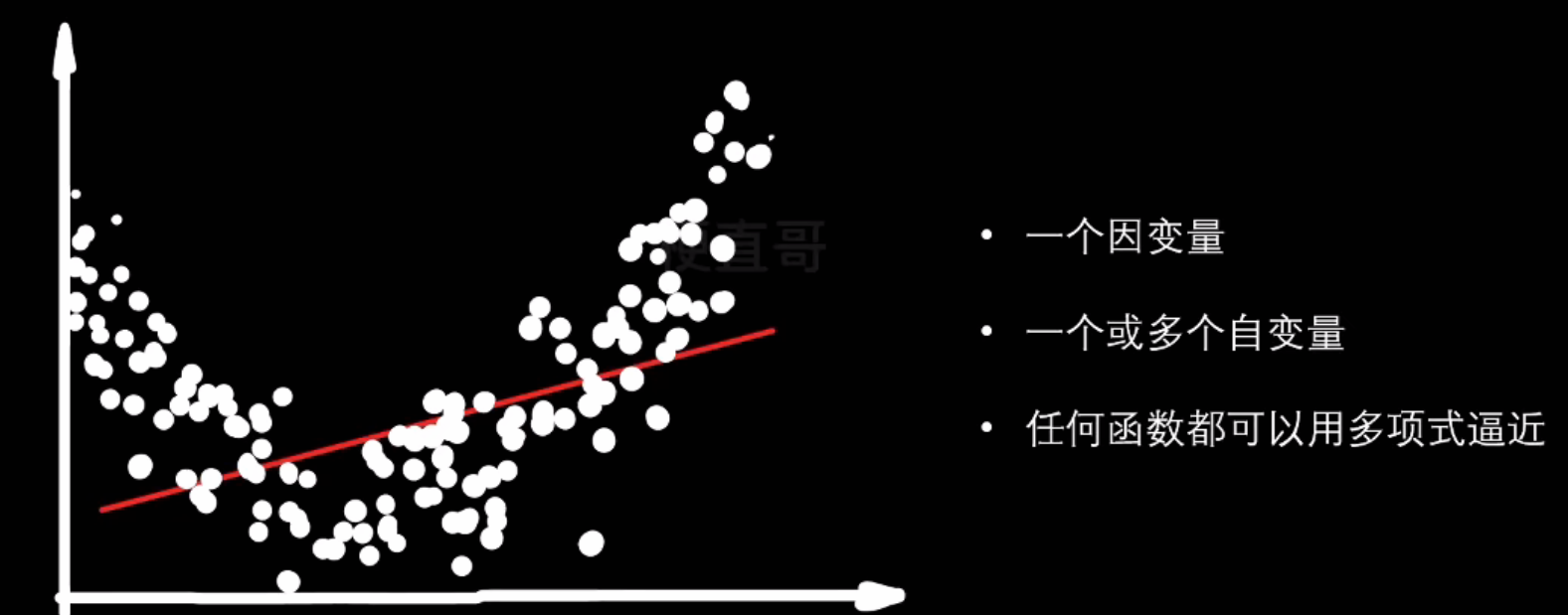
- 回归任务
- 线性回归
- 多项式回归
- 逻辑回归
分类和回归都是监督学习,因为二者的数据集都有标签,有直接的反馈
- 机器学习分类
分类依据

按训练数据中是否有标签(以及反馈信号的类型)分:
- 监督学习
- 分类和回归
- 训练数据有标记
- 基础且重要
- 无监督学习
- 训练数据未经标记
- 聚类:K均值算法(K-means),密度聚类(DBSCAN),最大期望算法
- 降维(主成分分析PCA,核方法)
- 关联规则学习:挖掘特征间关联关系,用Apriori方法和Eclat方法
- 半监督学习
- 少量标记数据
- 大量无标记数据
- 强化学习
- 观测环境,估计状态,执行操作,获得回报或惩罚
按 学习方式/数据输入方式 来分
- 批量学习
- 先训练再使用,需要大量的时间和计算资源
- 通常是离线完成
- 在线学习
- 循序渐进,边学边用

按怎么泛化来分
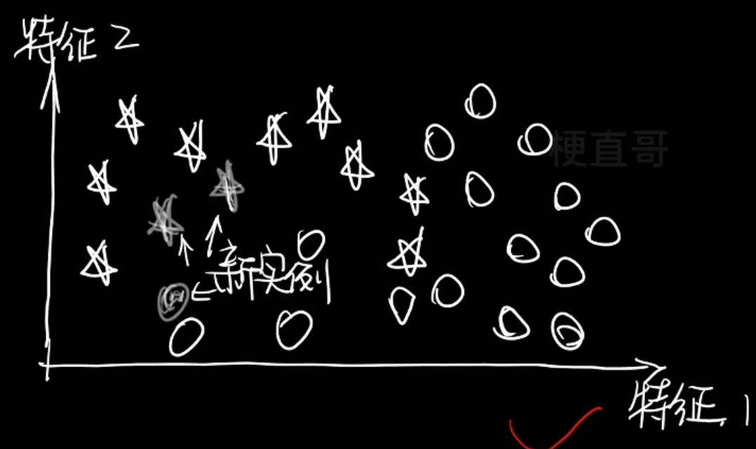
- 基于实例的学习
- 不同的泛化方式,先记住训练实例
- 相似度的学习
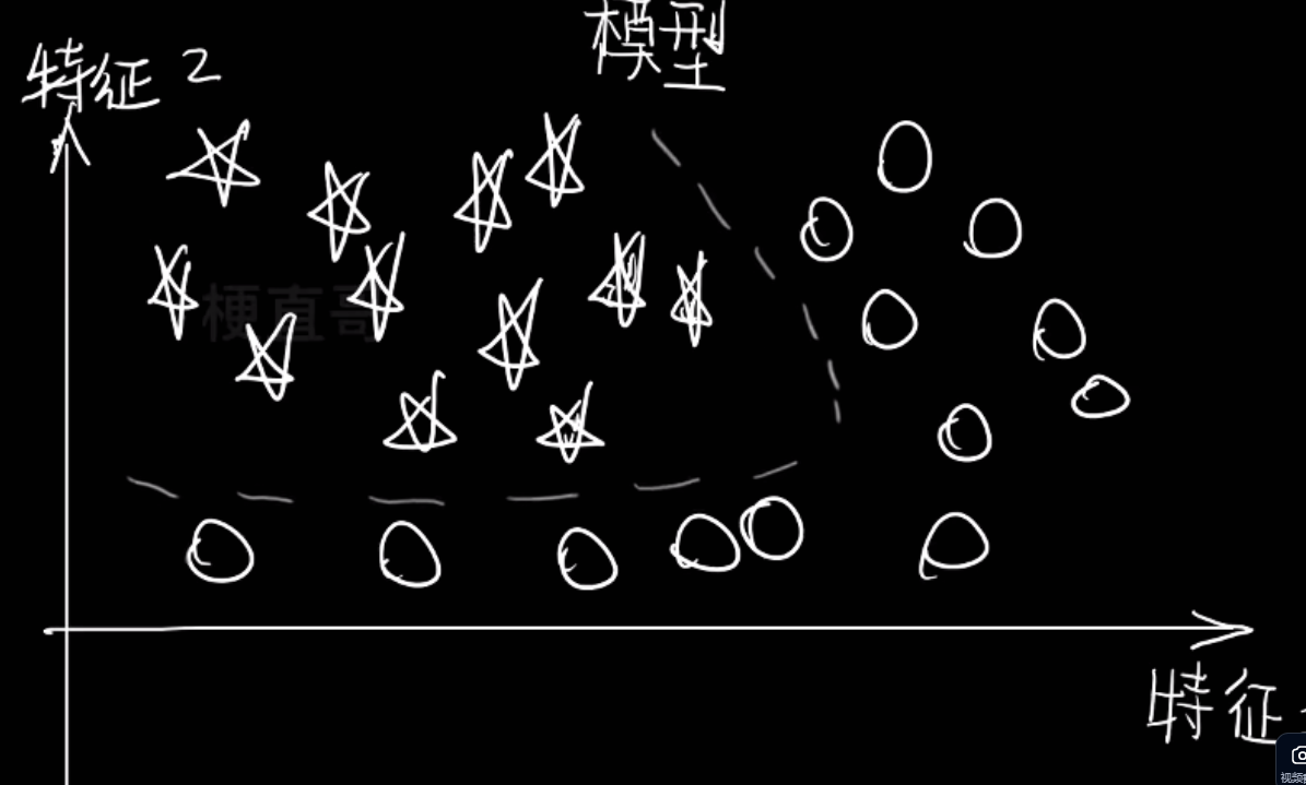
- 基于模型的学习
- 先构建模型,然后预测
- 常见误区
- 数据不是越多越好,多并不意味着准确,传统算法依旧有用
- 模型训练出来不一定可用, 深度学习是个黑盒子
- 机器学习本质是统计,确定性依旧很重要,我们要平衡好随机与确定性的平衡
- 机器学习适合大数据,很多问题天然小数据,小样本学习是挑战也是机会
- 机器学习尚在判断阶段,抽象思维和逻辑推理远未实现
- 自动驾驶伤了人算谁的错,机器的道德规范是什么
- 机器学习不死,深度学习局限性很大,其本质是空间几何变换
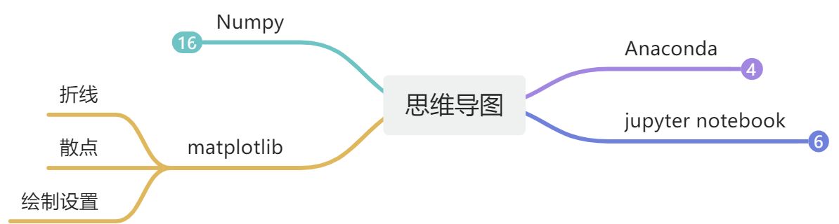
- 软件的使用
- Anaconda命令行
- conda -V
- 更新conda update conda
- 查看有多少个虚拟环境:conda env list
- 创建虚拟环境:conda create -n 名字 python=3.10
- 激活环境:conda activate 名字
- 查看当前环境已经安装的包:conda list
- 装包:conda install 包名
- 删除包:conda uninstall 包名
- 装可视化界面:conda install jupyter notebook
- 启动:jupyter notebook
- 删除安装的虚拟环境:conda deactivate(先退出创建的虚拟环境),conda remove -n 名字 --all
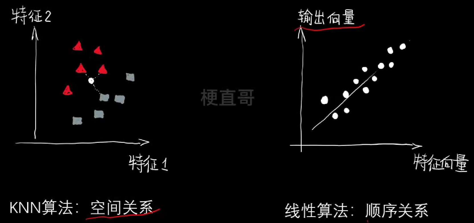
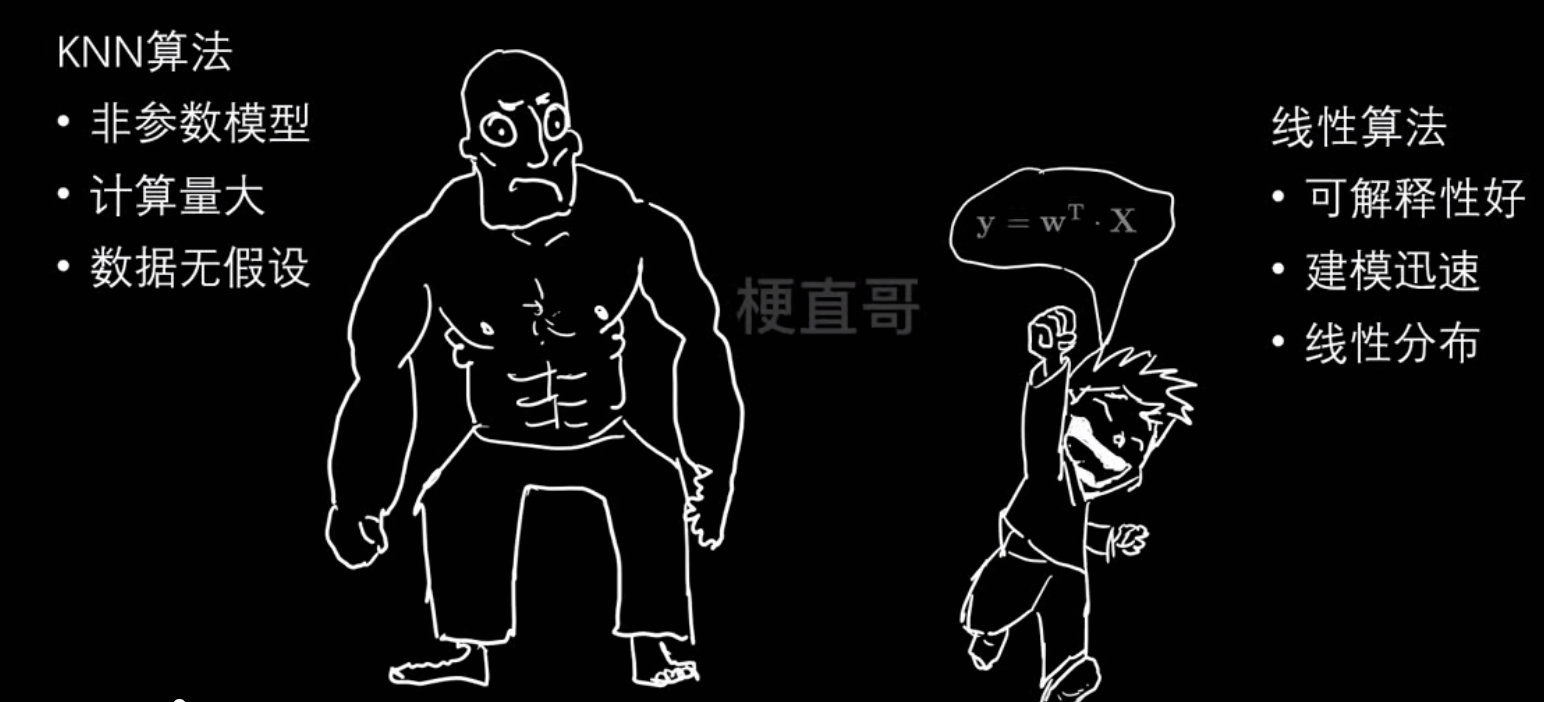
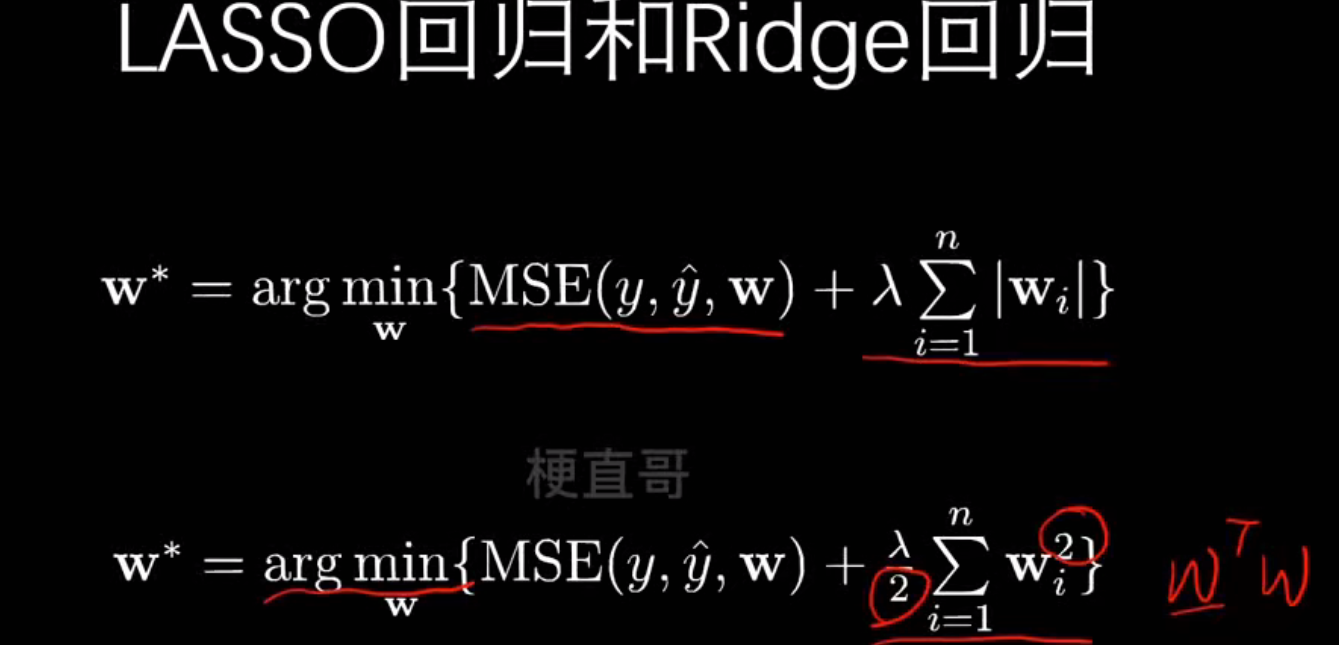
2、线性算法
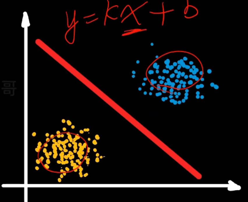
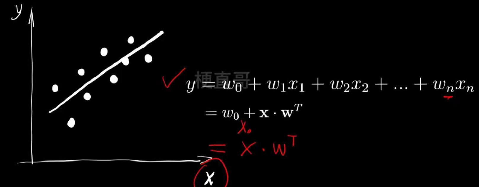
回归就是找条线
| 类型 | 代表算法 | 主要功能 | 损失函数 | 特点 |
|---|---|---|---|---|
| 回归任务 | 线性回归(Linear Regression) | 预测连续值(如房价、气温) | 均方误差(MSE) | 最经典的线性模型 |
| 岭回归(Ridge Regression) | 回归 + L2正则化 | MSE + λ‖w‖² | 抑制过拟合 | |
| 分类任务 | 逻辑回归(Logistic Regression) | 二分类(如生存/死亡) | 交叉熵损失 | “回归”名字但做分类 |
| 线性判别分析(LDA) | 二分类或多分类 | 最大化类间方差比 | 有概率解释 |
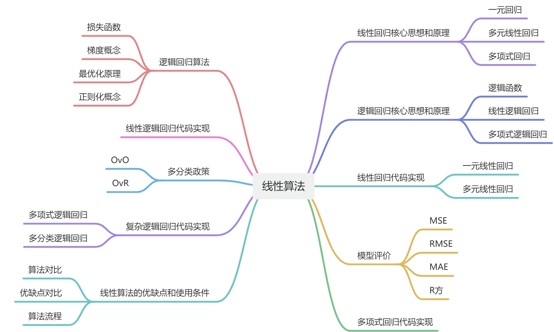
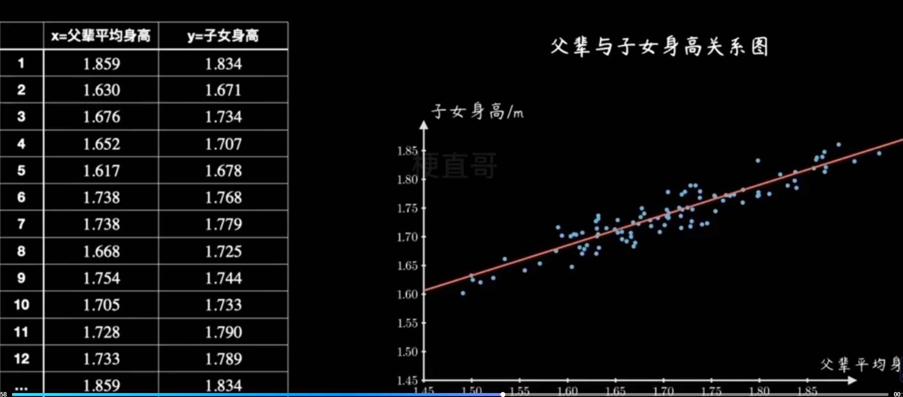
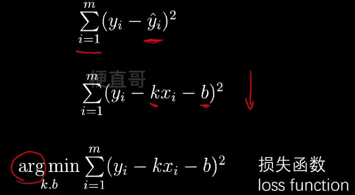
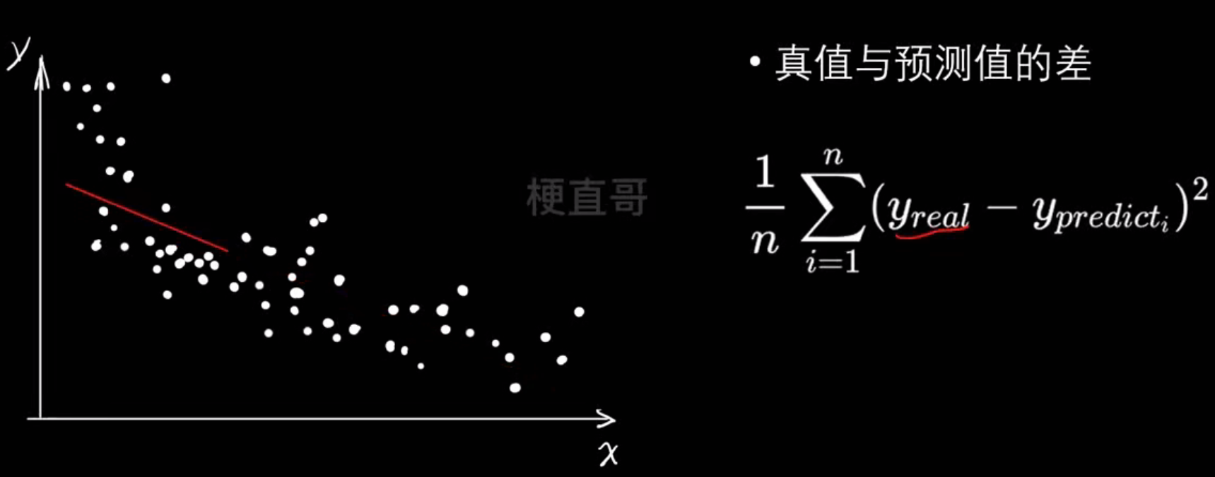
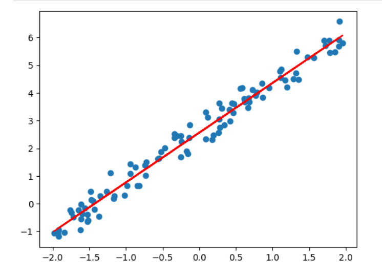
线性回归
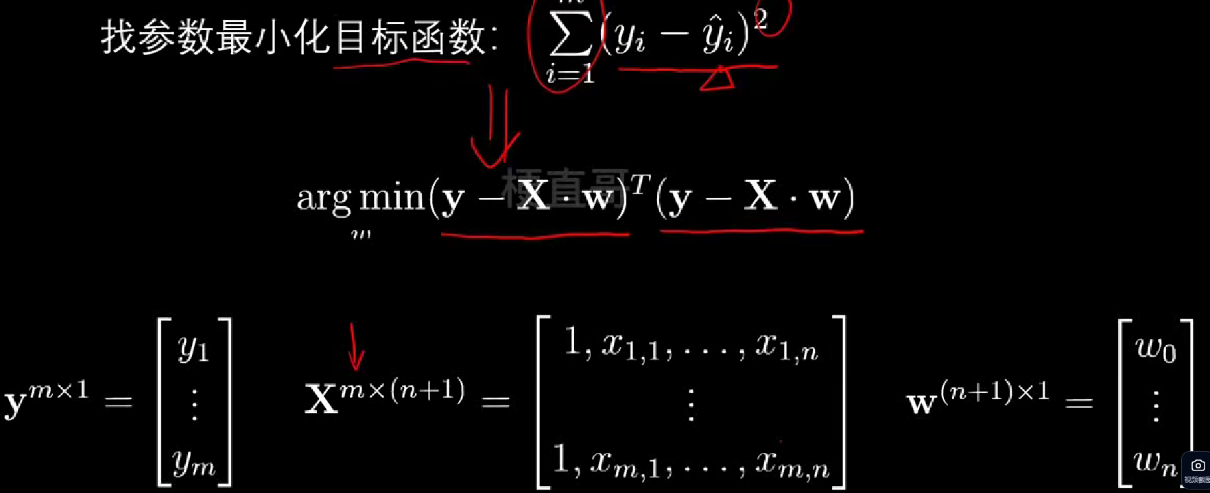
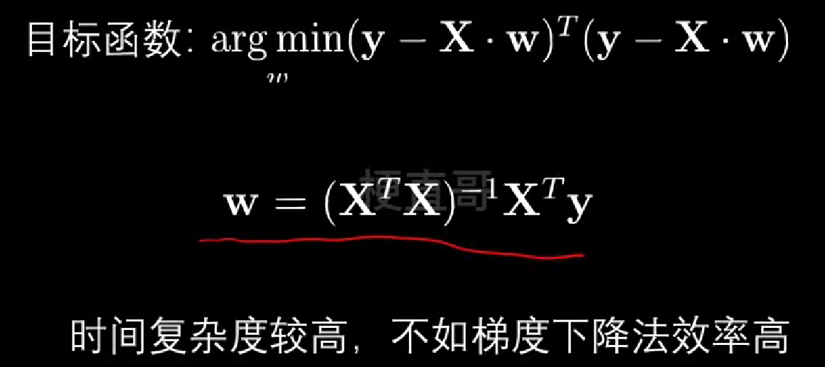
- 距离“误差”
- 损失函数
- 最优化
先导入数据集
import numpy as np
from sklearn import datasets
import matplotlib.pyplot as plt
import warnings
from sklearn.model_selection import train_test_split
from sklearn.linear_model import LinearRegression
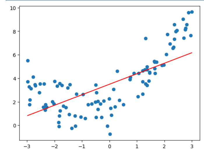
from sklearn.preprocessing import StandardScalerwarnings.filterwarnings("ignore")housing = datasets.fetch_california_housing()print(housing.DESCR)# 选择第一个特征(中位数收入)作为一元线性回归的特征
x = housing.data[:, 0] # MedInc - 中位数收入
y = housing.target# 限制数据范围以便更好地展示
x = x[y < 5]
y = y[y < 5]plt.scatter(x, y)
plt.xlabel('Median Income')
plt.ylabel('House Price')
plt.title('California Housing: Income vs Price')
plt.show()# 数据分割
x_train, x_test, y_train, y_test = train_test_split(x, y, test_size=0.3, random_state=0)plt.scatter(x_train, y_train)
plt.xlabel('Median Income')
plt.ylabel('House Price')
plt.title('Training Data')
plt.show()
- 一元线性回归
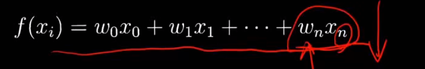
y=kx+b
最优化问题,民主投票,距离的衡量
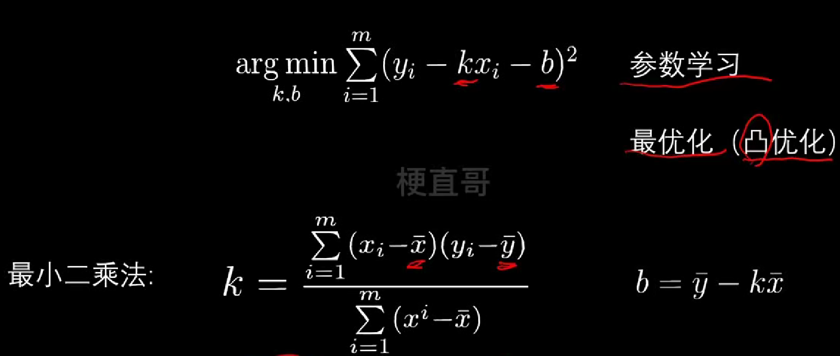
代码实现
- 一元线性回归公式实现
##
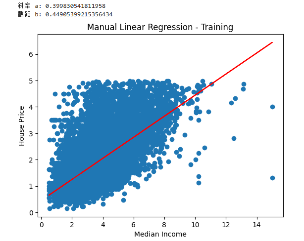
def fit(x, y):a_up = np.sum((x - np.mean(x)) * (y - np.mean(y)))a_bottom = np.sum((x - np.mean(x)) ** 2)a = a_up / a_bottomb = np.mean(y) - a * np.mean(x)return a, ba, b = fit(x_train, y_train)
print(f"斜率 a: {a}")
print(f"截距 b: {b}")plt.scatter(x_train, y_train)
plt.plot(x_train, a * x_train + b, c='r')
plt.xlabel('Median Income')
plt.ylabel('House Price')
plt.title('Manual Linear Regression - Training')
plt.show()
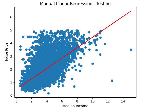
用测试集试试效果
plt.scatter(x_test, y_test)
plt.plot(x_test, a * x_test + b, c='r')
plt.xlabel('Median Income')
plt.ylabel('House Price')
plt.title('Manual Linear Regression - Testing')
plt.show()
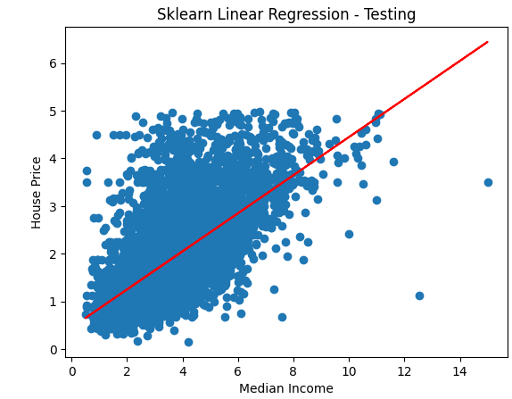
- sklearn实现一元线性回归
## sklearn实现一元线性回归
lin_reg = LinearRegression()
# reshape(-1, 1) 把一维数组变成二维数组
lin_reg.fit(x_train.reshape(-1, 1), y_train)y_predict = lin_reg.predict(x_test.reshape(-1, 1))plt.scatter(x_test, y_test)
plt.plot(x_test, y_predict, c='r')
plt.xlabel('Median Income')
plt.ylabel('House Price')
plt.title('Sklearn Linear Regression - Testing')
plt.show()
- 多元线性回归
## sklearn 实现多元线性回归
# 使用所有特征
x_multi = housing.data
y_multi = housing.target# 限制数据范围
x_multi = x_multi[y_multi < 5]
y_multi = y_multi[y_multi < 5]x_train_multi, x_test_multi, y_train_multi, y_test_multi = train_test_split(x_multi, y_multi, test_size=0.3, random_state=0
)lin_reg_multi = LinearRegression()
lin_reg_multi.fit(x_train_multi, y_train_multi)score = lin_reg_multi.score(x_test_multi, y_test_multi)
print(f"多元线性回归 R² 分数: {score}")输出:
多元线性回归 R² 分数: 0.5582591396048222
此处不需要归一化,没啥区别
因为多元线性回归学习的是每个特征的权重(系数),模型会自动调整这些权重来适应不同特征的数据尺度
## 归一化
standardScaler = StandardScaler()
standardScaler.fit(x_train_multi)
x_train_scaled = standardScaler.transform(x_train_multi)
x_test_scaled = standardScaler.transform(x_test_multi)lin_reg_scaled = LinearRegression()
lin_reg_scaled.fit(x_train_scaled, y_train_multi)score_scaled = lin_reg_scaled.score(x_test_scaled, y_test_multi)
print(f"归一化后多元线性回归 R² 分数: {score_scaled}")输出:
归一化后多元线性回归 R² 分数: 0.5582591396048212
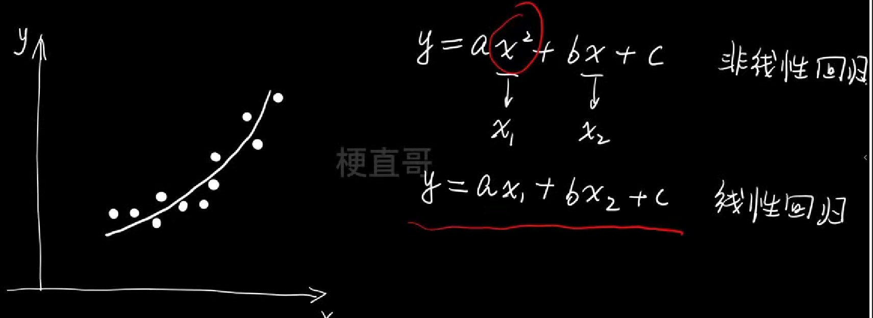
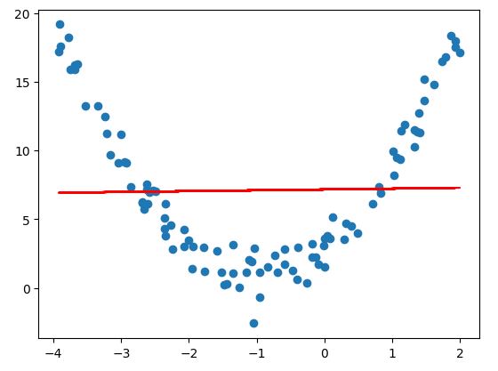
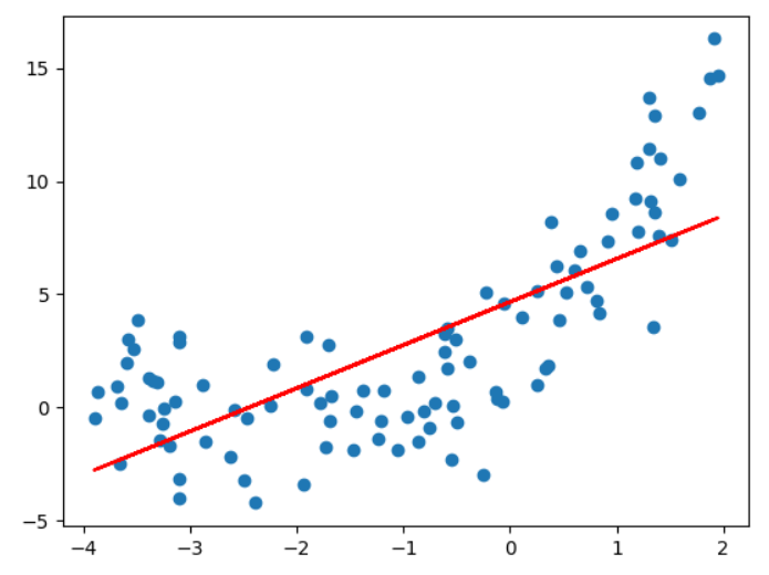
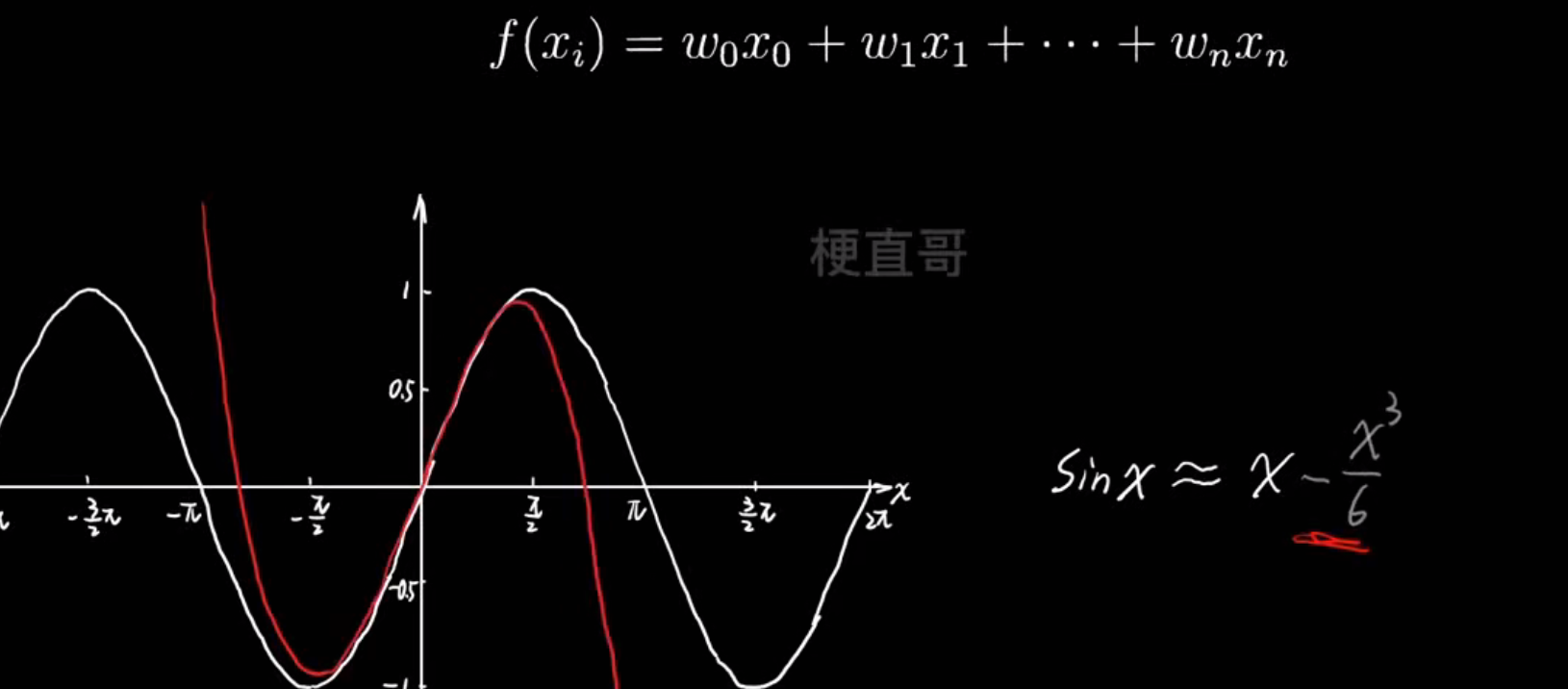
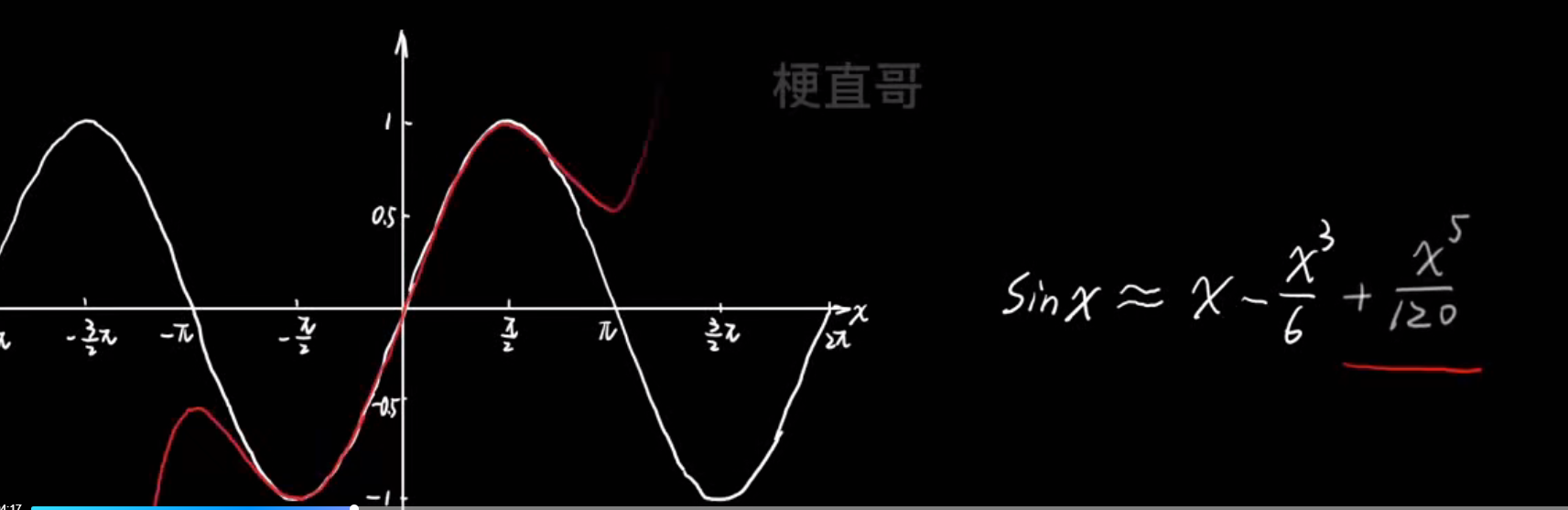
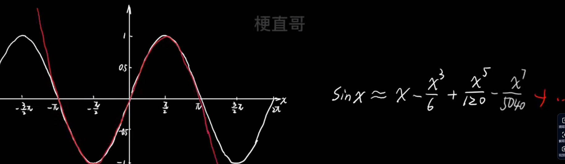
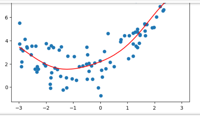
多项式回归
import numpy as np
import matplotlib.pyplot as plt
# 构造非线性数据
x = np.random.uniform(-4,2,size=(100))
y = 2*x**2 + 4*x + 3 + np.random.randn(100)
X = x.reshape(-1,1)
plt.scatter(x,y)
plt.show()
#线性回归
from sklearn.linear_model import LinearRegression
linear_regression = LinearRegression()
linear_regression.fit(X,y)
y_predict = linear_regression.predict(X)
plt.scatter(x,y)
plt.plot(x,y_predict,color='red')
plt.show()
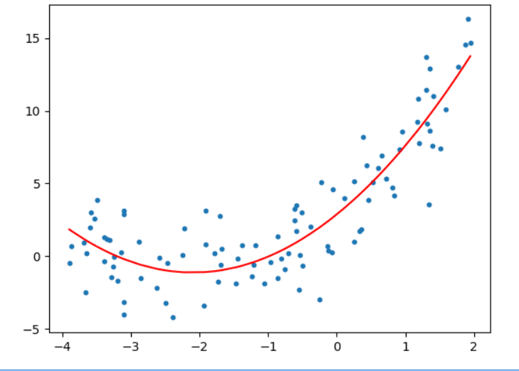
# 多项式回归
X[:5]
X_new = np.hstack([X,X**2])
X_new[:5]
linear_regression_new = LinearRegression()
linear_regression_new.fit(X_new,y)
y_predict_new = linear_regression_new.predict(X_new)
plt.scatter(x,y)
plt.plot(np.sort(x),y_predict_new[np.argsort(x)],color="red")
plt.show()
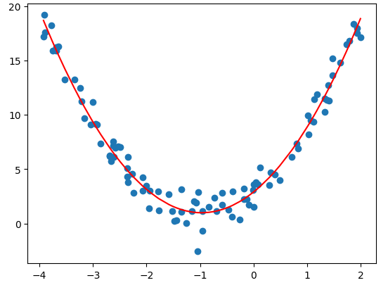
# 函数的截距
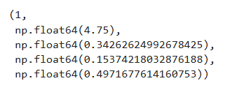
linear_regression_new.intercept_
# 特征值
linear_regression_new.coef_输出:
np.float64(2.910763300495222)
array([3.93855269, 2.02866524])
# scikit-learn中的PolynomialFeatures
from sklearn.preprocessing import PolynomialFeatures
polynomial_features = PolynomialFeatures(degree=2)
X_poly = polynomial_features.fit_transform(X)
X_poly[:5]输出:
array([[ 1.        , -2.62673044,  6.89971278],[ 1.        , -0.40289062,  0.16232085],[ 1.        , -2.35268823,  5.53514189],[ 1.        ,  1.00887873,  1.01783629],[ 1.        ,  1.8734883 ,  3.5099584 ]])
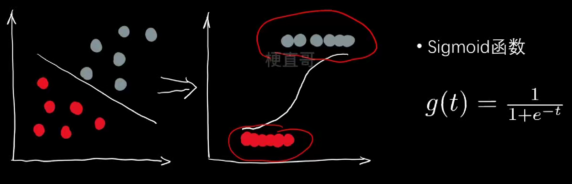
逻辑回归
叫着回归的名,做着分类的活
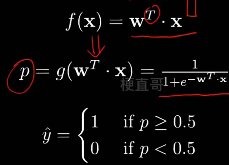
- 线性逻辑回归
逻辑函数(Logistic Function):
# 生成训练集
import numpy as np
import matplotlib.pyplot as plt
from sklearn.model_selection import train_test_split
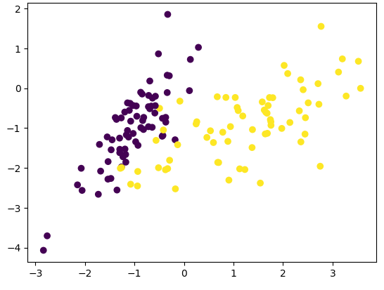
from sklearn.datasets import make_classificationx, y = make_classification(n_samples=200,n_features=2,n_redundant=0,n_classes=2,n_clusters_per_class=1,random_state=1024
)
x.shape, y.shape
x_train, x_test, y_train, y_test = train_test_split(x, y, train_size = 0.7, random_state = 233, stratify = y)
plt.scatter(x_train[:,0], x_train[:,1], c = y_train)
plt.show()
# sklearn中的逻辑回归
from sklearn.linear_model import LogisticRegression
clf = LogisticRegression()
clf.fit(x_train, y_train)
clf.score(x_train, y_train)   #0.9357142857142857
clf.score(x_test, y_test)     #0.95
clf.predict(x_test)
输出:
array([1, 0, 1, 0, 1, 1, 1, 1, 1, 0, 1, 1, 0, 0, 0, 0, 0, 1, 0, 0, 0, 1,0, 0, 1, 0, 0, 1, 0, 0, 0, 1, 1, 0, 0, 1, 0, 0, 0, 1, 0, 1, 0, 1,0, 1, 0, 0, 1, 1, 1, 0, 1, 0, 1, 1, 0, 0, 1, 0])
# 属于每个类别的概率
clf.predict_proba(x_test)
# 取概率最大的类别索引(即预测类别)
np.argmax(clf.predict_proba(x_test), axis = 1)
输出:
array([1, 0, 1, 0, 1, 1, 1, 1, 1, 0, 1, 1, 0, 0, 0, 0, 0, 1, 0, 0, 0, 1,0, 0, 1, 0, 0, 1, 0, 0, 0, 1, 1, 0, 0, 1, 0, 0, 0, 1, 0, 1, 0, 1,0, 1, 0, 0, 1, 1, 1, 0, 1, 0, 1, 1, 0, 0, 1, 0])
# 超参数调优
# 用 网格搜索(GridSearchCV) 自动尝试多组超参数组合,找到让模型效果最好的那一组
from sklearn.model_selection import GridSearchCV
params = [{'penalty': ['l2', 'l1'],'C': [0.0001, 0.001, 0.01, 0.1, 1, 10, 100, 1000],'solver': ['liblinear']
}, {'penalty': ['none'],'C': [0.0001, 0.001, 0.01, 0.1, 1, 10, 100, 1000],'solver': ['lbfgs']
}, {'penalty': ['elasticnet'],'C': [0.0001, 0.001, 0.01, 0.1, 1, 10, 100, 1000],'l1_ratio': [0, 0.25, 0.5, 0.75, 1],'solver': ['saga'],'max_iter': [200]
}]
grid = GridSearchCV(estimator=LogisticRegression(),param_grid=params,n_jobs=-1
)
grid.fit(x_train, y_train)
grid.best_score_   #np.float64(0.95)
grid.best_estimator_.score(x_test, y_test)  #0.9333333333333333
grid.best_params_
输出:
{'C': 1,'l1_ratio': 0.75,'max_iter': 200,'penalty': 'elasticnet','solver': 'saga'}
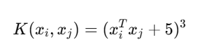
- 多项式逻辑回归:
生成数据集
import numpy as np
import matplotlib.pyplot as plt
from sklearn.model_selection import train_test_split
from sklearn.datasets import make_classification
np.random.seed(0)
X = np.random.normal(0,1,size=(200,2))
y = np.array((X[:,0]**2)+(X[:,1]**2)<2, dtype='int')
y
输出:
array([0, 0, 0, 1, 1, 0, 1, 1, 0, 1, 0, 1, 0, 1, 0, 1, 0, 1, 0, 1, 0, 0,1, 0, 0, 1, 1, 1, 1, 1, 1, 0, 1, 0, 1, 1, 0, 1, 1, 1, 0, 0, 0, 1,0, 1, 1, 1, 0, 1, 0, 0, 0, 1, 0, 0, 0, 1, 1, 1, 1, 1, 1, 0, 1, 1,1, 1, 1, 1, 0, 1, 0, 0, 1, 0, 1, 1, 0, 1, 0, 1, 0, 0, 1, 1, 1, 1,1, 1, 0, 0, 0, 1, 0, 1, 1, 1, 1, 0, 1, 1, 0, 1, 1, 1, 1, 1, 1, 0,1, 1, 0, 1, 1, 0, 1, 1, 0, 1, 1, 1, 0, 0, 0, 1, 1, 1, 0, 0, 1, 1,0, 1, 1, 0, 0, 1, 1, 0, 1, 0, 1, 0, 0, 1, 0, 1, 1, 1, 0, 1, 1, 0,1, 1, 1, 1, 1, 1, 1, 1, 1, 0, 1, 1, 1, 0, 0, 0, 1, 1, 1, 1, 1, 0,0, 1, 0, 1, 1, 1, 1, 1, 1, 1, 1, 1, 0, 1, 0, 0, 0, 0, 0, 1, 0, 1,0, 0])x_train, x_test, y_train, y_test = train_test_split(X, y, train_size = 0.7, random_state = 233, stratify = y)
plt.scatter(x_train[:,0], x_train[:,1], c = y_train)
plt.show()
多项式逻辑回归代码实现:
from sklearn.preprocessing import PolynomialFeatures
poly = PolynomialFeatures(degree=2)
poly.fit(x_train)
x2 = poly.transform(x_train)
x2t = poly.transform(x_test)
clf.fit(x2, y_train)
clf.score(x2, y_train)  # 1.0
clf.score(x2t, y_test)  # 0.9666666666666667
线性回归的模型评价
有误差怎么办?
# 加州房价预测模型(线性回归 + 模型评估 + 可视化)
import numpy as np
import matplotlib.pyplot as plt
from sklearn.datasets import fetch_california_housing
from sklearn.model_selection import train_test_split
from sklearn.preprocessing import StandardScaler
from sklearn.linear_model import LinearRegression
from sklearn.metrics import mean_squared_error, mean_absolute_error, r2_scoredata = fetch_california_housing()
X = data.data
y = data.targetX_train, X_test, y_train, y_test = train_test_split(X, y, test_size=0.25, random_state=42)scaler = StandardScaler()
X_train = scaler.fit_transform(X_train)
X_test = scaler.transform(X_test)model = LinearRegression()
model.fit(X_train, y_train)y_pred = model.predict(X_test)mse = mean_squared_error(y_test, y_pred)
rmse = np.sqrt(mse)
mae = mean_absolute_error(y_test, y_pred)
r2 = r2_score(y_test, y_pred)print("===== 加州房价预测模型评价 =====")
print(f"均方误差 (MSE): {mse:.4f}")
print(f"均方根误差 (RMSE): {rmse:.4f}")
print(f"平均绝对误差 (MAE): {mae:.4f}")
print(f"决定系数 (R²): {r2:.4f}")输出:
均方误差 (MSE): 0.5411
均方根误差 (RMSE): 0.7356
平均绝对误差 (MAE): 0.5297
决定系数 (R²): 0.5911
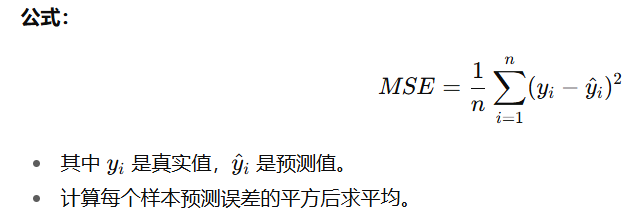
- 均方误差(MSE, Mean Squared Error)
特点:
- 误差平方会放大大偏差样本的影响 → 对“极端错误”更敏感。
- 单位是“平方单位”(在这里是房价平方,解释上不直观)。
解读结果:
MSE = 0.5411
→ 模型预测值与真实房价的平均平方偏差约为 0.54(单位约是“十万美元²”)。
- 均方根误差(RMSE, Root Mean Squared Error)
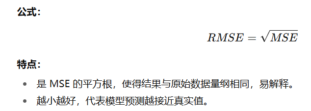
解读结果:
RMSE = 0.7356
→ 模型平均预测误差约为 0.73 个房价单位(约 $73,000 左右)。
可理解为:模型的预测结果平均偏差在 ±7 万美元上下。
- 平均绝对误差(MAE, Mean Absolute Error)
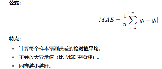
解读结果:
MAE = 0.5297
→ 模型平均每个样本预测偏差约 0.53 个房价单位(≈ $53,000)。
相当于:平均每套房预测误差大概五万美元上下。
- 决定系数(R², Coefficient of Determination)
解读结果:
R² = 0.5911
→ 模型能解释房价变化中 约 59% 的方差,剩下 41% 由未建模的因素(非线性关系、特征缺失等)决定。
| 指标 | 含义 | 理想情况 | 你的结果 | 说明 |
|---|---|---|---|---|
| MSE | 平方误差平均 | 越小越好 | 0.5411 | 整体误差适中 |
| RMSE | 与原单位一致的均方误差 | 越小越好 | 0.7356 | 平均预测误差约 $73,000 |
| MAE | 平均绝对误差 | 越小越好 | 0.5297 | 平均偏差约 $53,000 |
| R² | 拟合优度 | 越接近1越好 | 0.5911 | 模型解释力中等偏上 |
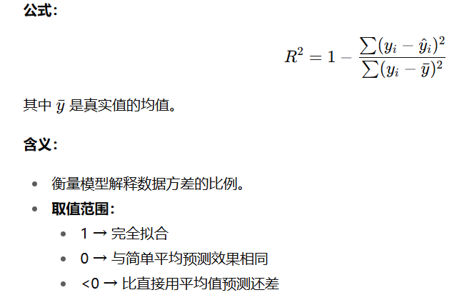
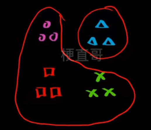
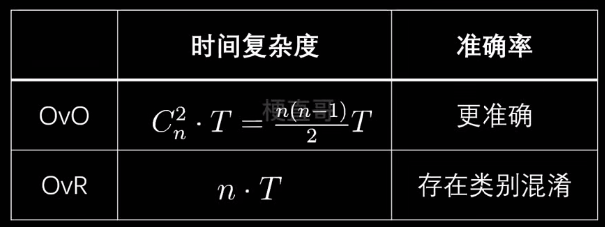
多分类策略
复杂问题简单化,把多分类问题转化为二分类问题:
- one vs one一对一-------- 每次对两个类别进行分类
如图有四组数据,每次拿出两个

一共可以分为六组
- one vs rest一对剩余------ 每次对一个类别 vs 其他所有类别
- 性能对比
生成数据集
from sklearn import datasets
iris = datasets.load_iris()
x = iris.data
y = iris.target
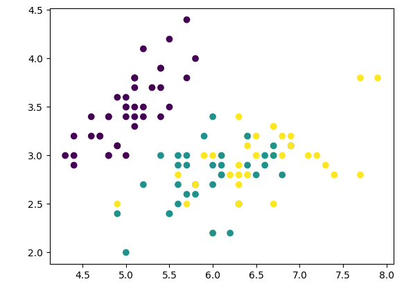
x_train, x_test, y_train, y_test = train_test_split(x, y, random_state=666)
plt.scatter(x_train[:,0], x_train[:,1], c=y_train)
plt.show()
# 一对一
from sklearn.multiclass import OneVsOneClassifierovr = OneVsOneClassifier(clf)
ovr.fit(x_train,y_train)
ovr.score(x_test, y_test)  # 1.0# 一对多
from sklearn.multiclass import OneVsRestClassifierovr = OneVsRestClassifier(clf)
ovr.fit(x_train,y_train)
ovr.score(x_test, y_test)  #0.9736842105263158
线性算法优缺点及使用条件
| 类别 | 线性回归 | 多项式回归 | 逻辑回归 |
|---|---|---|---|
| 数学表达式 |  | 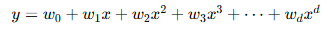 | 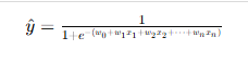 |
| 模型类型 | 回归(预测连续值) | 回归(预测连续值,非线性) | 分类(预测0/1概率) |
| 可视化示意 | 一条直线拟合数据 (线性趋势) | 一条弯曲的平滑曲线 (可拟合非线性关系) | 一条S形曲线(Sigmoid) (输出0~1概率) |
| 优点 | 1. 模型简单、易理解 2. 建模和训练速度快 | 1. 能拟合非线性数据 2. 学习能力更强 3. 在合适阶数下表现优越 | 1. 模型清晰,参数解释性强 2. 输出有概率意义 3. 计算量小,可在线学习 4. 可处理过拟合(L1/L2正则) |
| 缺点 | 1. 对异常值敏感 2. 无法表达复杂模式 3. 仅能拟合线性关系 | 1. 阶数选择不当易过拟合 2. 对异常值仍敏感 3. 特征数量急剧增加 | 1. 只能用于分类问题 2. 特征空间大时性能下降 3. 处理特征相关性较差 |
| 适用场景 | 数据趋势接近线性时,如房价~面积 | 变量间存在非线性关系,如温度~时间、销量价格曲线 | 二分类任务,如垃圾邮件识别、疾病预测、客户流失判断 |
| 核心思想 | 找一条直线,使预测值与真实值差距最小 | 用线性模型在高维空间近似非线性关系 | 使用 Sigmoid 将线性结果映射为概率,进行分类 |
| 输出形式 | 连续值(实数) | 连续值(平滑曲线) | 概率值(0~1) |
3、核心概念精讲
机器学习干啥的:

四种语言的转换:


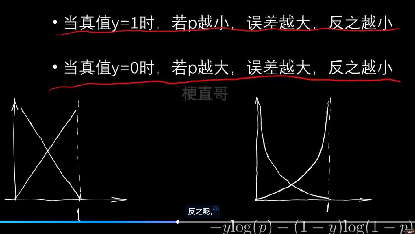
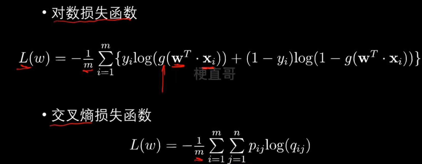
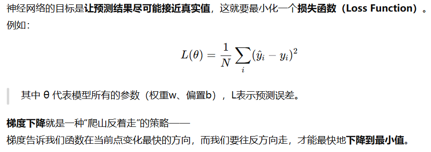
损失函数
缘由:
- 机器学习的本质是在数据中找规律
- 先假定带参数的模型
- 数据投票打分的数学描述
- Loss function/cost function
损失函数:针对不同情况下用不同标准来衡量样本和模型之间的损失
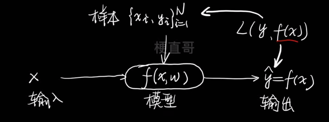
损失函数越小,说明效果越好
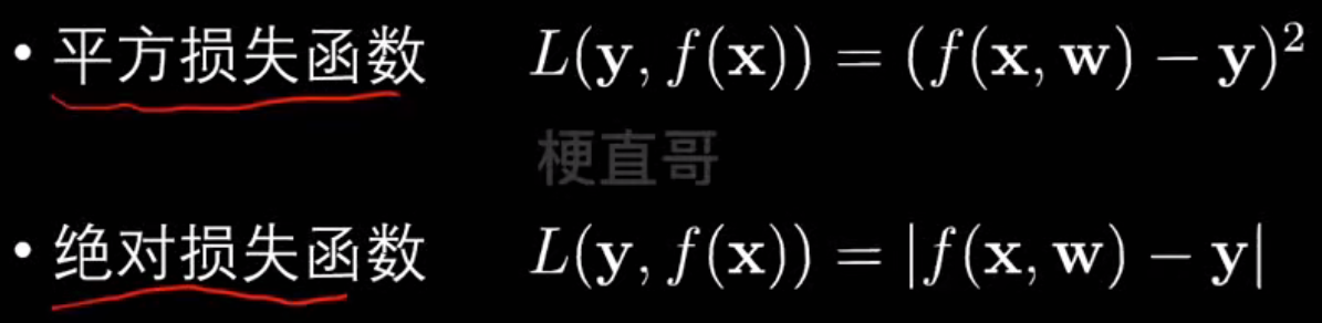
常见损失函数:
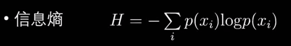
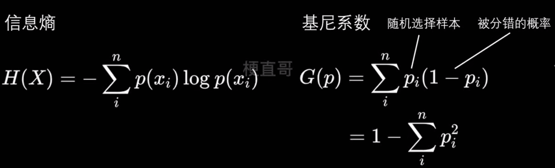
什么是熵?
- 衡量混乱程度
- 熵增定律
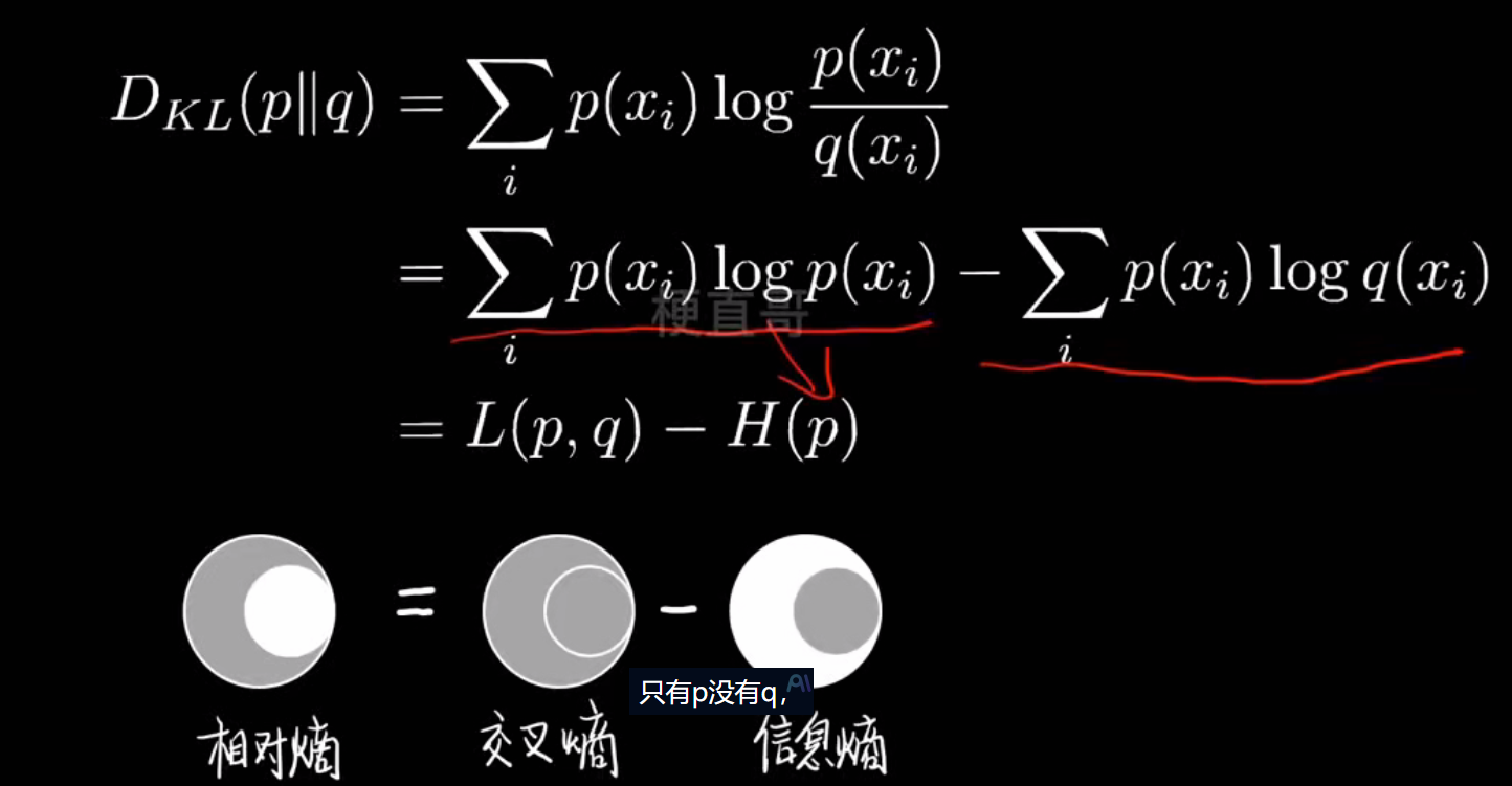
交叉熵直观解释:
交叉熵就是一个 衡量两个概率分布差异的指标,差距越大,交叉熵越大
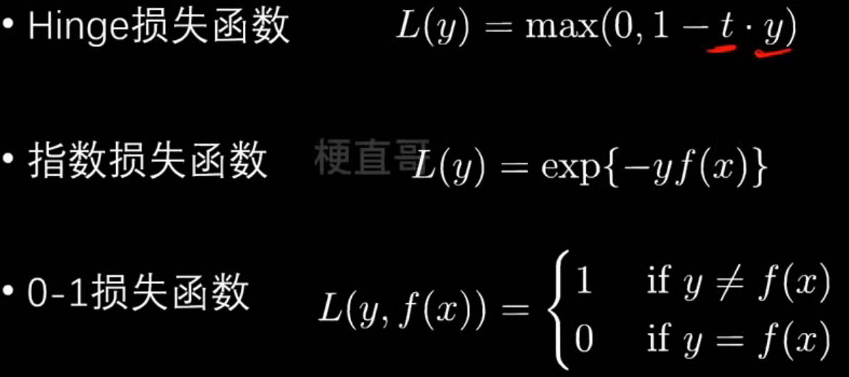
其他损失函数
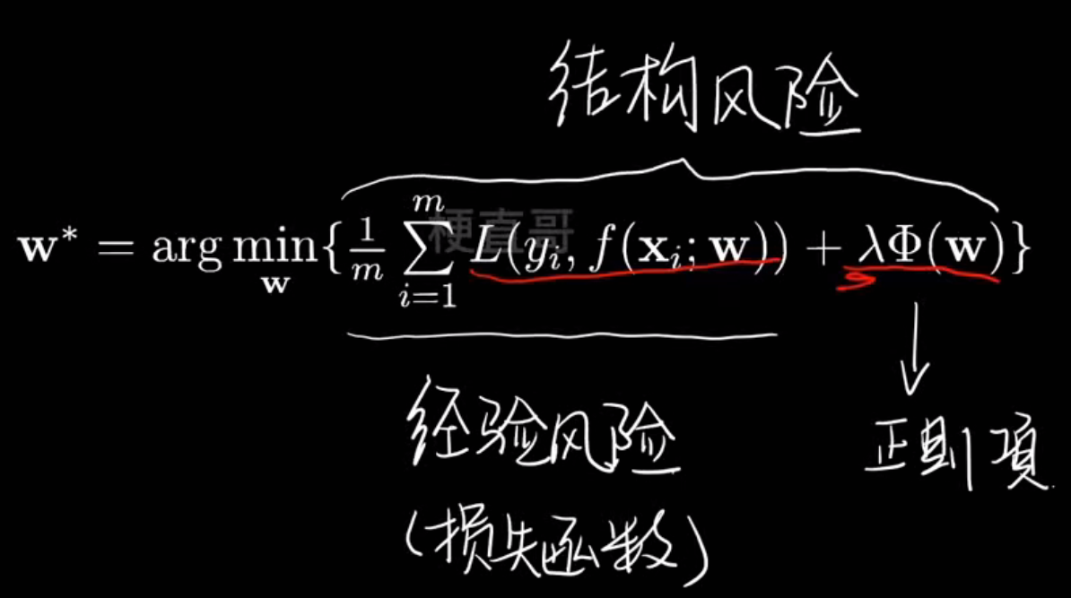
| 对比项 | 经验风险最小化 (ERM) | 结构风险最小化 (SRM) |
|---|---|---|
| 思想核心 | 让训练误差最小 | 让“训练误差 + 模型复杂度”总和最小 |
| 是否防过拟合 | 容易过拟合 | 可以抑制过拟合 |
| 数学形式 | 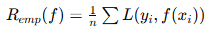 | 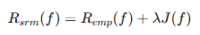 |
| 典型算法 | 普通线性回归、KNN | 岭回归、LASSO、SVM |
| 惩罚项 | 无 | 有,如 ( |
| 理论基础 | 统计学习的经验逼近 | Vapnik 的 VC 维理论(模型容量控制) |
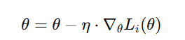
梯度下降

这是一种最优化算法,为了 找到一组参数 w,b,让损失函数 L的值最小
如图,显然最低点的时候损失最小
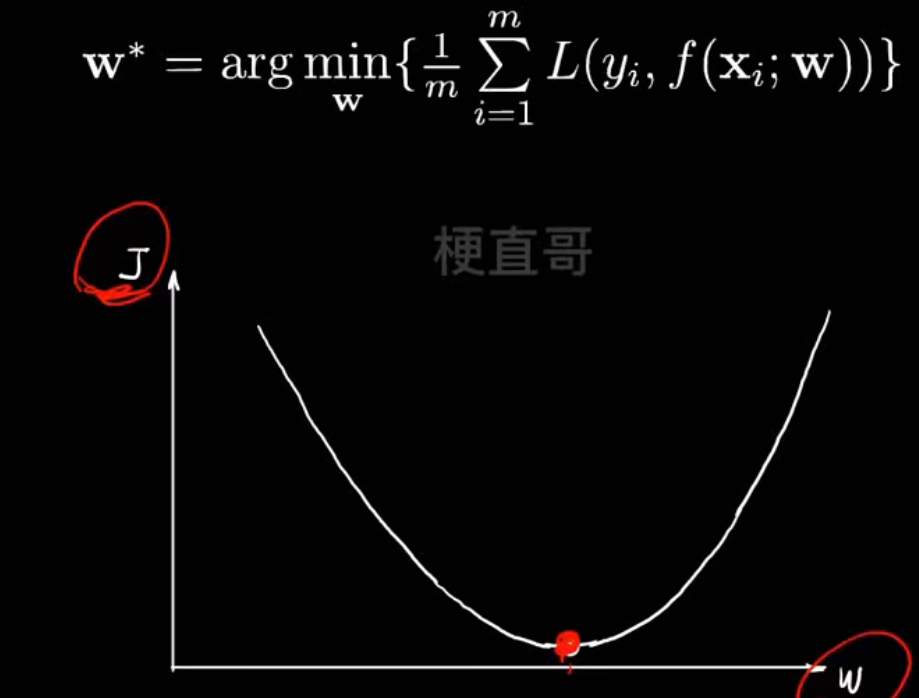
那么怎么找到这个最低点呢?
用搜索策略
这是最优化的核心
确定好搜索方向和搜索速度
梯度(Gradient)就是函数曲面陡度,偏导数是具体方向的陡度,梯度是所有方向偏导数向量和
学习率:
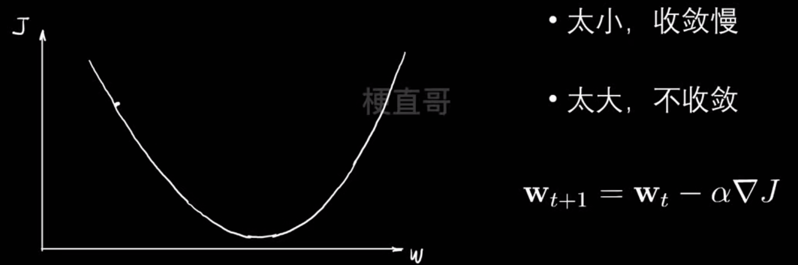
梯度下降过程中往往极值点不止一个,辨析局部最优和全局最优
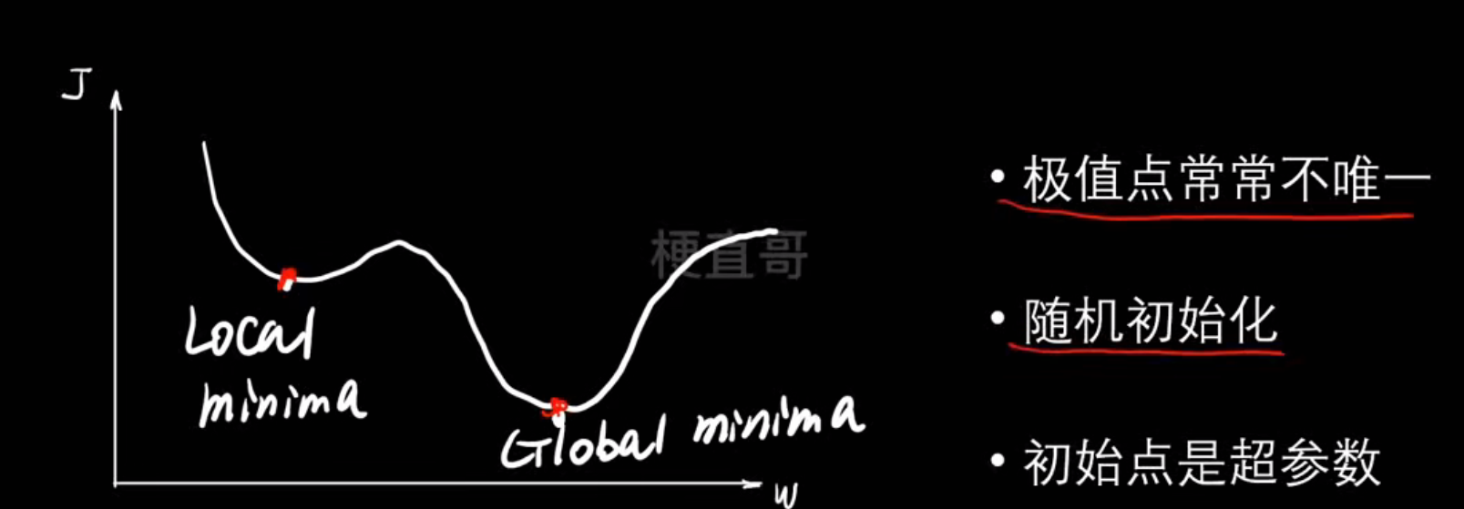
寻找最低点的过程中陷入局部最优,于是我们需要寻找更好的下山办法:
- AdaGrad → 每个参数独立学习率
- RMSProp → 防止学习率衰减过快
- AdaDelta → 自动调节学习率
- Adam → 综合优点,最常用
常见梯度下降算法:
| 方法 | 每次迭代样本量 | 优点 | 缺点 | 典型应用 |
|---|---|---|---|---|
| 批量梯度下降(BGD) | 全部样本 | 收敛稳定、结果精确 | 计算量大、内存占用高 | 小数据集或离线训练 |
| 随机梯度下降(SGD) | 1个样本 | 更新快、可跳出局部最优 | 收敛不稳定、震荡大 | 在线学习、流式数据 |
| 小批量梯度下降(Mini-Batch) | 部分样本(如32~256) | 稳定高效、支持并行 | 批量大小需调参 | 深度学习主流方法 |
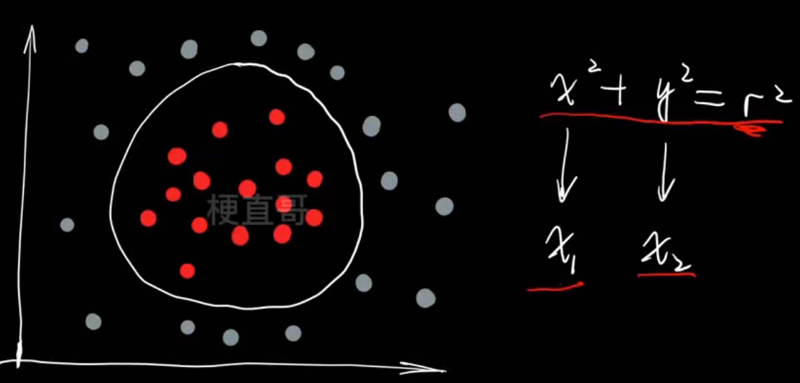
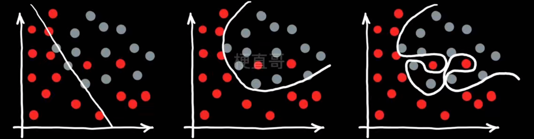
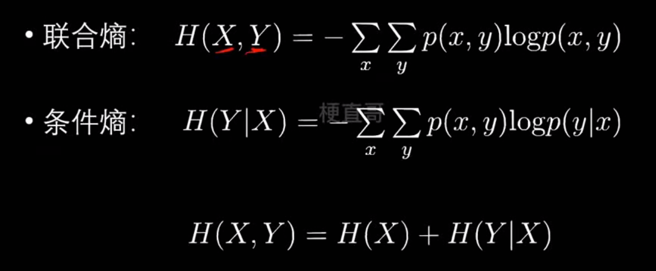
决策边界
分类模型如何描绘决策边界
决策边界是模型将不同类别区分开的分界线(或曲面)。换句话说,它定义了模型在输入空间中“判定类别”的临界位置。
不同算法的决策边界
| 模型类型 | 决策边界形状 | 举例说明 |
|---|---|---|
| 线性模型(如 Logistic Regression, Linear SVM) | 直线(二维)或超平面(高维) | 用线性方程 ( w^T x + b = 0 ) 划分空间 |
| 非线性模型(如 Kernel SVM, 决策树, 神经网络) | 曲线或复杂曲面 | 可以弯曲、折叠甚至形成多个区域 |
| k近邻(KNN) | 不规则边界 | 取决于样本分布,边界会非常“碎” |
| 神经网络 | 随层数增加可学到非常复杂的非线性边界 | CNN、MLP 等深层模型能逼近任意形状的边界 |
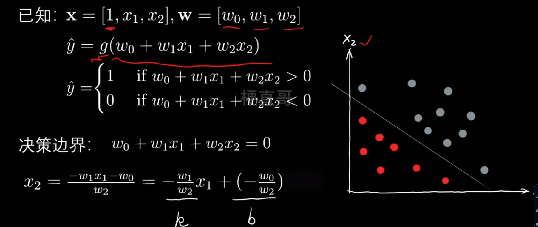
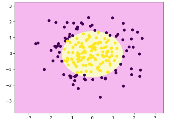
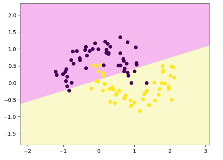
举个例子:
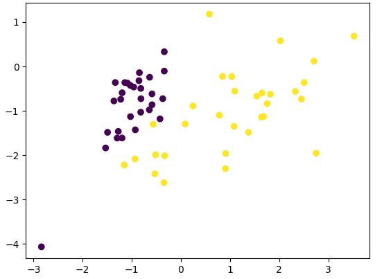
规则边界绘制:
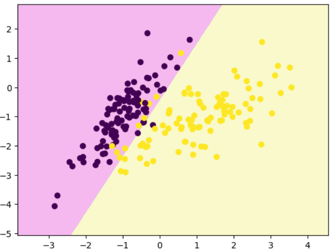
# 线性逻辑回归决策边界
import numpy as np
import matplotlib.pyplot as plt
from sklearn.model_selection import train_test_split
from sklearn.datasets import make_classification
from sklearn.linear_model import LogisticRegressionx,y=make_classification(n_samples=200,n_features=2,n_redundant=0,n_classes=2,n_clusters_per_class=1,random_state=1024
)
x_train,x_test,y_train,y_test=train_test_split(x,y,test_size=0.7,random_state=24)
clf=LogisticRegression()
clf.fit(x_train,y_train)
clf.score(x_train,y_train) #0.9333333333333333
plt.scatter(x_train[:,0],x_train[:,1],c=y_train)
plt.show()
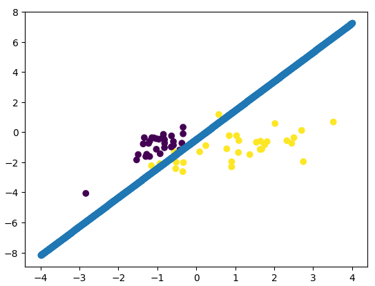
clf.coef_ # # 权重 w,array([[ 2.51671784, -1.3052424 ]])
clf.intercept_ # 截距 b,array([-0.61049327])
x1=np.linspace(-4,4,1000)
x2=(-clf.coef_[0][0]*x1-clf.intercept_)/clf.coef_[0][1]
plt.scatter(x_train[:,0],x_train[:,1],c=y_train)
# 决策边界
plt.scatter(x1,x2)
plt.show()
# 决策边界绘制函数
def decision_boundary_plot(X, y, clf):axis_x1_min, axis_x1_max = X[:,0].min() - 1, X[:,0].max() + 1axis_x2_min, axis_x2_max = X[:,1].min() - 1, X[:,1].max() + 1x1, x2 = np.meshgrid( np.arange(axis_x1_min,axis_x1_max, 0.01) , np.arange(axis_x2_min,axis_x2_max, 0.01))z = clf.predict(np.c_[x1.ravel(),x2.ravel()])z = z.reshape(x1.shape)from matplotlib.colors import ListedColormapcustom_cmap = ListedColormap(['#F5B9EF','#BBFFBB','#F9F9CB'])plt.contourf(x1, x2, z, cmap=custom_cmap)plt.scatter(X[:,0], X[:,1], c=y)plt.show()decision_boundary_plot(x,y,clf)
不规则边界绘制:
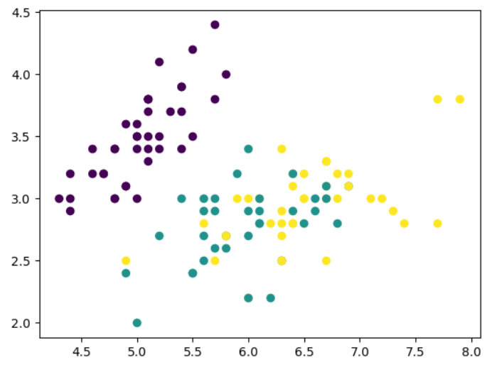
# 三分类
from sklearn import datasets
iris=datasets.load_iris()
x=iris.data[:,:2]
y=iris.target
x_train,x_test,y_train,y_test=train_test_split(x,y,random_state=666)
plt.scatter(x_train[:,0],x_train[:,1],c=y_train)
plt.show()
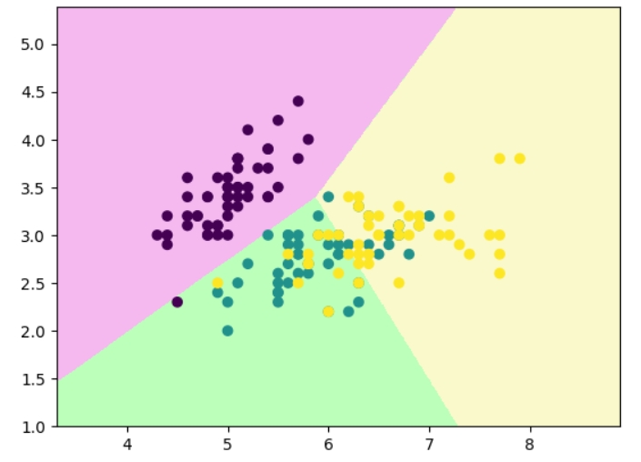
# 三分类的决策边界
clf.fit(x_train,y_train)
clf.score(x_test,y_test)   #0.7894736842105263
decision_boundary_plot(x,y,clf)
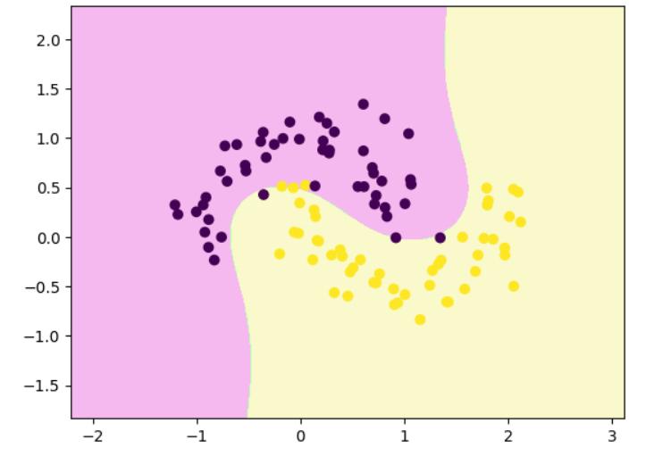
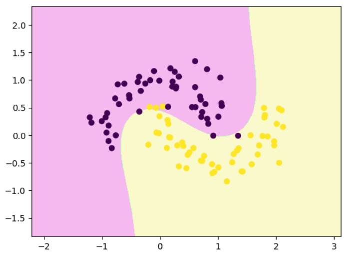
# 多项式逻辑回归
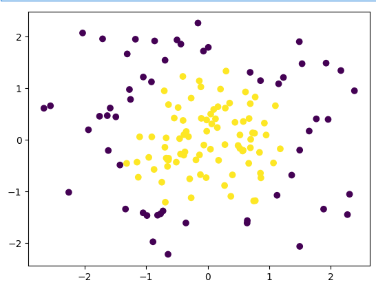
np.random.seed(0)
x = np.random.normal(0, 1, size=(200, 2))
y = np.array((x[:,0]**2+x[:,1]**2)<2, dtype='int')
x_train, x_test, y_train, y_test = train_test_split(x, y, train_size = 0.7, random_state = 233, stratify = y)
plt.scatter(x_train[:,0], x_train[:,1], c = y_train)
plt.show()
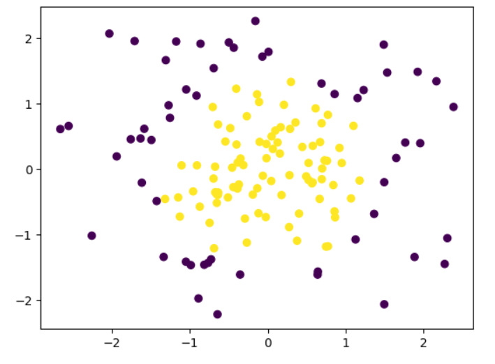
# 多项式逻辑回归的决策边界
from sklearn.pipeline import Pipeline
from sklearn.preprocessing import PolynomialFeatures
from sklearn.preprocessing import StandardScaler
from sklearn.linear_model import LogisticRegressionclf_pipe=Pipeline([('poly',PolynomialFeatures(degree=2)),('std_scaler',StandardScaler()),('log_reg',LogisticRegression())
])
clf_pipe.fit(x_train,y_train)
decision_boundary_plot(x,y,clf_pipe)
过拟合和欠拟合
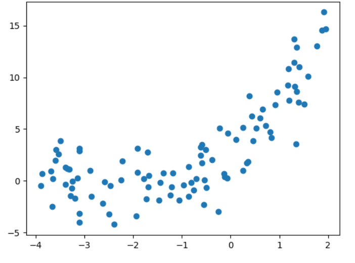
# 数据集
import numpy as np
import matplotlib.pyplot as pltnp.random.seed(233)
x=np.random.uniform(-4,2,size=(100))
y=x**2+4*x+3+2*np.random.randn(100)
X=x.reshape(-1,1)plt.scatter(x,y)
plt.show()

# 欠拟合
from sklearn.linear_model import LinearRegression
linear_regression=LinearRegression()
linear_regression.fit(X,y)
y_predict=linear_regression.predict(X)
plt.scatter(x,y)
plt.plot(x,y_predict,color='red')
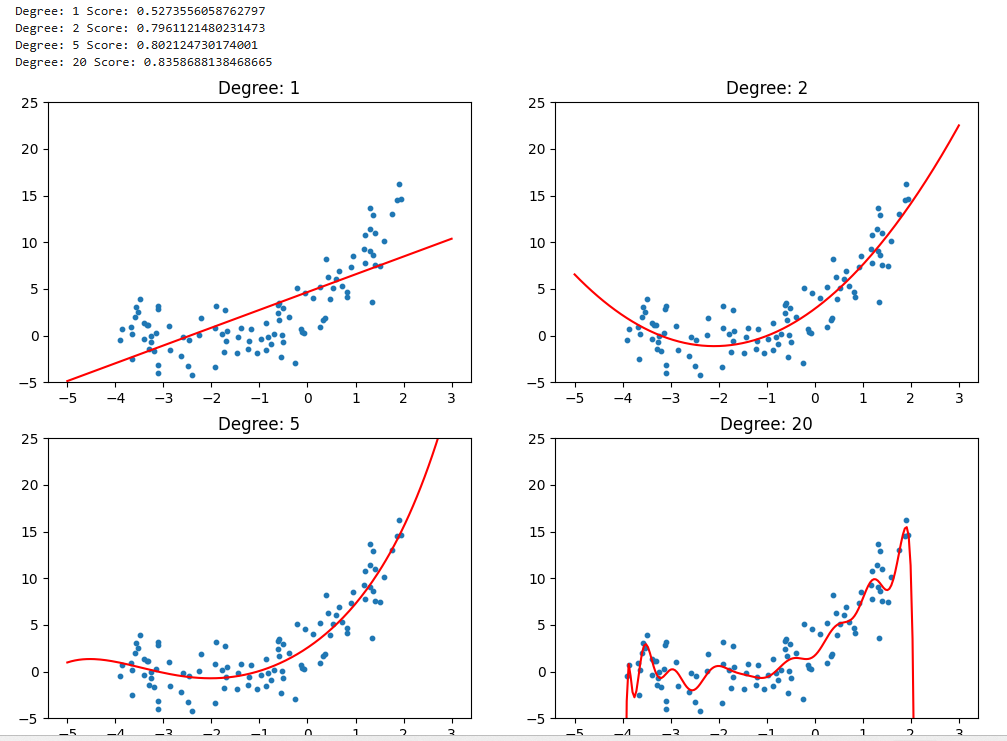
plt.show()linear_regression.score(X,y) #0.5273556058762796
# 过拟合
from sklearn.preprocessing import PolynomialFeatures
polynomial_features=PolynomialFeatures(degree=2)
X_poly=polynomial_features.fit_transform(X)linear_regression=LinearRegression()
linear_regression.fit(X_poly,y)y_predict=linear_regression.predict(X_poly)plt.scatter(x,y,s=10)
plt.plot(np.sort(x),y_predict[np.argsort(x)],color='red')
plt.show()
# 多项式回归另一种方法
X_new=np.linspace(-5,3,200).reshape(-1,1)
X_new_poly=polynomial_features.fit_transform(X_new)
y_predict=linear_regression.predict(X_new_poly)plt.scatter(x,y,s=10)
plt.plot(X_new,y_predict,color='red')
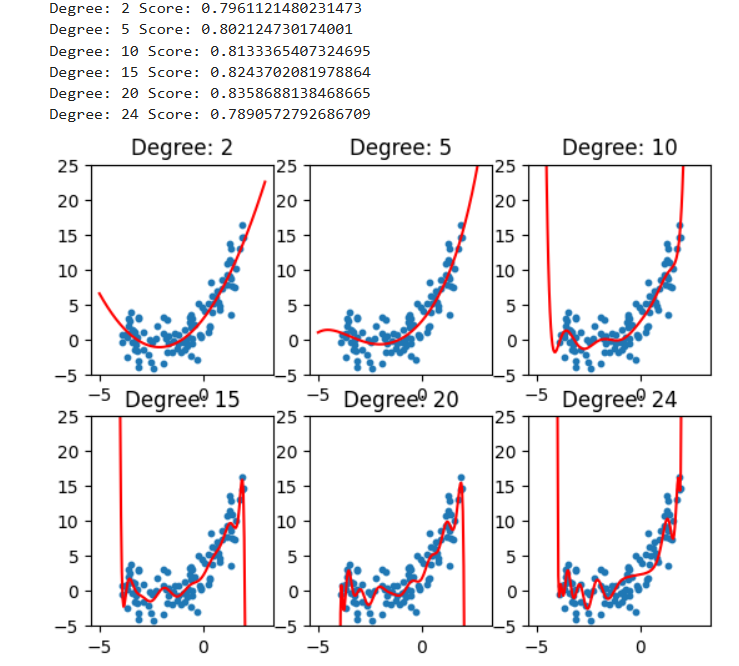
plt.show()print("Degree:",2,"Score:",linear_regression.score(X_poly,y)) #Degree: 2 Score: 0.7961121480231473
# 绘制不同degree效果
degrees=[2,5,10,15,20,24]
for i, degree in enumerate(degrees):polynomial_features = PolynomialFeatures(degree = degree)X_poly = polynomial_features.fit_transform(X)linear_regression = LinearRegression()linear_regression.fit(X_poly, y)X_new = np.linspace(-5, 3, 200).reshape(-1, 1)X_new_poly = polynomial_features.fit_transform(X_new)y_predict = linear_regression.predict(X_new_poly)plt.subplot(2, 3, i + 1)plt.title("Degree: {0}".format(degree))plt.scatter(x, y, s = 10)plt.ylim(-5, 25)plt.plot(X_new, y_predict, color = 'red')print("Degree:", degree, "Score:", linear_regression.score(X_poly, y))plt.show()
学习曲线
过拟合老要画曲线太麻烦了,我们通过学习曲线去评判拟合效果更简单
学习曲线就是:随着训练数据量增加,模型性能(误差或准确率)的变化曲线
什么是学习曲线?
它通常包含两条曲线:
- 训练集曲线:模型在训练数据上的表现;
- 验证集/测试集曲线:模型在新数据上的表现
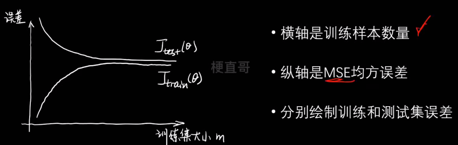
| 情况 | 特征 | 含义 |
|---|---|---|
| 欠拟合(Underfitting) | 训练误差高,测试误差也高,且两者都几乎不下降 | 模型太简单,学不到规律 |
| 过拟合(Overfitting) | 训练误差很低,但测试误差高,两条曲线差距大 | 模型太复杂,记住了训练数据 |
| 拟合良好 | 两条曲线都低,并且趋于接近 | 模型复杂度合适、泛化好 |
# 数据集
import numpy as np
import matplotlib.pyplot as pltnp.random.seed(233)
x=np.random.uniform(-4,2,size=(100))
y=x**2+4*x+3+2*np.random.randn(100)
X=x.reshape(-1,1)plt.scatter(x,y)
plt.show()
# 线性回归和多项式回归
from sklearn.linear_model import LinearRegression
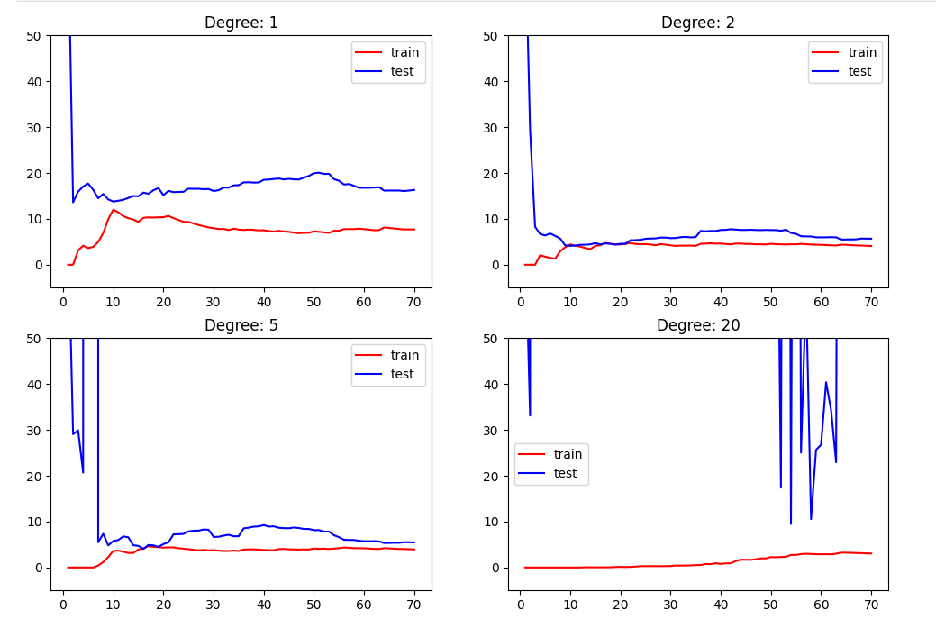
from sklearn.preprocessing import PolynomialFeaturesplt.rcParams["figure.figsize"] = (12, 8)degrees = [1, 2, 5, 20]
for i, degree in enumerate(degrees):polynomial_features = PolynomialFeatures(degree = degree)X_poly = polynomial_features.fit_transform(X)linear_regression = LinearRegression()linear_regression.fit(X_poly, y)X_new = np.linspace(-5, 3, 200).reshape(-1, 1)X_new_poly = polynomial_features.fit_transform(X_new)y_predict = linear_regression.predict(X_new_poly)plt.subplot(2, 2, i + 1)plt.title("Degree: {0}".format(degree))plt.scatter(x, y, s = 10)plt.ylim(-5, 25)plt.plot(X_new, y_predict, color = "red")print("Degree:", degree, "Score:", linear_regression.score(X_poly, y))plt.show()
# 划分数据集
from sklearn.model_selection import train_test_split
x_train,x_test,y_train,y_test=train_test_split(x,y,train_size=0.7,random_state=233)x_train.shape,x_test.shape,y_train.shape,y_test.shape输出:
((70,), (30,), (70,), (30,))
# 学习曲线
from sklearn.metrics import mean_squared_errorplt.rcParams["figure.figsize"] = (12, 8)degrees = [1, 2, 5, 20]
for i, degree in enumerate(degrees):polynomial_features = PolynomialFeatures(degree = degree)X_poly_train = polynomial_features.fit_transform(x_train.reshape(-1, 1))X_poly_test = polynomial_features.fit_transform(x_test.reshape(-1, 1))train_error, test_error = [], []for k in range(len(x_train)):linear_regression = LinearRegression()linear_regression.fit(X_poly_train[:k + 1], y_train[:k + 1])y_train_pred = linear_regression.predict(X_poly_train[:k + 1])train_error.append(mean_squared_error(y_train[:k + 1], y_train_pred))y_test_pred = linear_regression.predict(X_poly_test)test_error.append(mean_squared_error(y_test, y_test_pred))plt.subplot(2, 2, i + 1)plt.title("Degree: {0}".format(degree))plt.ylim(-5, 50)plt.plot([k + 1 for k in range(len(x_train))], train_error, color = "red", label = 'train')plt.plot([k + 1 for k in range(len(x_train))], test_error, color = "blue", label = 'test')plt.legend()plt.show()
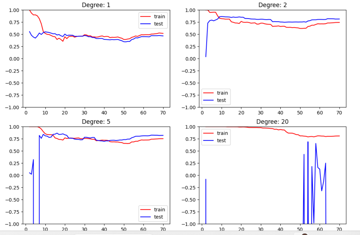
from sklearn.metrics import mean_squared_errorplt.rcParams["figure.figsize"] = (12, 8)degrees = [1, 2, 5, 20]
for i, degree in enumerate(degrees):polynomial_features = PolynomialFeatures(degree = degree)X_poly_train = polynomial_features.fit_transform(x_train.reshape(-1, 1))X_poly_test = polynomial_features.fit_transform(x_test.reshape(-1, 1))train_error, test_error = [], []for k in range(1, len(x_train)):linear_regression = LinearRegression()linear_regression.fit(X_poly_train[:k + 1], y_train[:k + 1])train_error.append(linear_regression.score(X_poly_train[:k + 1], y_train[:k + 1]))test_error.append(linear_regression.score(X_poly_test, y_test))plt.subplot(2, 2, i + 1)plt.title("Degree: {0}".format(degree))plt.ylim(-1, 1)plt.plot([k + 1 for k in range(1, len(x_train))], train_error, color = "red", label = 'train')plt.plot([k + 1 for k in range(1, len(x_train))], test_error, color = "blue", label = 'test')plt.legend()plt.show()
| 指标 | 含义 | 越什么越好 | 单位 |
|---|---|---|---|
| MSE(Mean Squared Error) | 预测值与真实值之间的平均平方差 | 越小越好 | 与原始数据单位的平方一致 |
| R²(Coefficient of Determination) | 模型能解释数据方差的比例(相对衡量) | 越大越好(上限1) | 无单位、相对指标 |
| 比较维度 | 第一版代码(用 mean_squared_error) | 第二版代码(用 model.score()) |
|---|---|---|
| 性能指标 | 使用 均方误差(MSE) 作为误差度量 | 使用 R² 决定系数 作为性能指标 |
| 纵轴含义 | “误差” 越低越好(下越好) | “拟合度” 越高越好(上越好) |
| 显示方向 | y轴是误差,越靠近 0 越优 | y轴是 R²,越靠近 1 越优 |
| 曲线趋势 | 下降曲线:随着样本增加误差下降 | 上升曲线:随着样本增加R²上升 |
| 用途偏向 | 直观展示“误差下降趋势” | 强调“模型解释能力提升” |
| 易于发现的问题 | 过拟合/欠拟合更直观(看误差间距) | 模型好坏更直观(看R²靠近1) |
| 底层计算 | 每次调用 mean_squared_error() | 每次调用 LinearRegression().score() |
| 数值取值范围 | MSE ≥ 0,无上限 | R² ∈ (-∞, 1] |
| 方向一致性 | 误差 ↓ → 模型更好 | R² ↑ → 模型更好 |
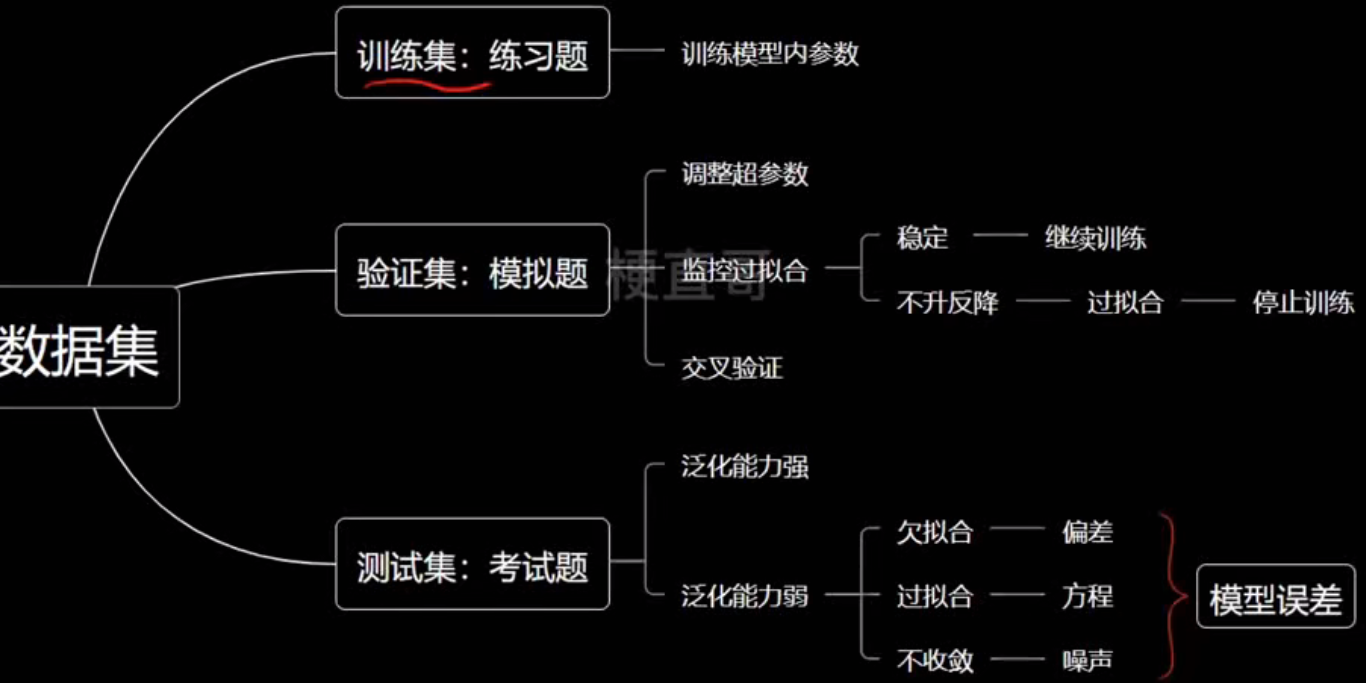
交叉验证
验证集:

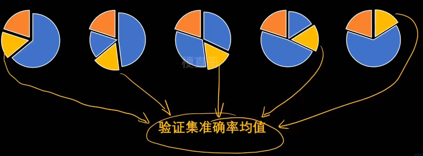
k-fold交叉验证:
┌──────────────────────────────┐
│  GridSearchCV 工作流程       │
│                              │
│  for 每一组超参:             │
│     for 每一折CV:            │
│         拆分训练/验证数据    │
│         训练模型 → 得分      │
│     平均折内得分             │
│  取平均分最高的超参组合       │
└──────────────────────────────┘
代码实现:
# 数据集
import numpy as np
from sklearn.model_selection import train_test_split
from sklearn.datasets import load_irisiris = load_iris()
x = iris.data
y = iris.targetx_train, x_test, y_train, y_test = train_test_split(x, y, train_size = 0.7, random_state = 233, stratify = y)
x_train.shape, x_test.shape, y_train.shape, y_test.shape输出:
((105, 4), (45, 4), (105,), (45,))
from sklearn.model_selection import cross_val_score
from sklearn.neighbors import KNeighborsClassifierneigh = KNeighborsClassifier()、
# 把训练集 x_train, y_train 分成 5 份(cv=5),
# 用 5 折交叉验证(5-Fold Cross Validation)评估模型性能。
cv_scores = cross_val_score(neigh, x_train, y_train, cv = 5)
print(cv_scores)输出:
[0.95238095 1.         0.95238095 0.85714286 1.        ]
| 轮次 | 训练集 | 验证集 |
|---|---|---|
| 第1次 | 折2~5 | 折1 |
| 第2次 | 折1,3,4,5 | 折2 |
| 第3次 | 折1,2,4,5 | 折3 |
| 第4次 | 折1,2,3,5 | 折4 |
| 第5次 | 折1,2,3,4 | 折5 |
每次:
- 模型用 4 份数据训练;
- 用剩下 1 份验证;
- 记录这次验证的准确率。
最后得到 5 个分数。
best_score = -1
best_n = -1
best_weight = ''
best_p = -1
best_cv_scores = None
for n in range(1, 20):for weight in ['uniform', 'distance']:for p in range(1, 7):neigh = KNeighborsClassifier(n_neighbors = n,weights = weight,p = p)cv_scores = cross_val_score(neigh, x_train, y_train, cv = 5)score = np.mean(cv_scores)if score > best_score:best_score = scorebest_n = nbest_weight = weightbest_p = pbest_cv_scores = cv_scoresprint("n_neighbors:", best_n)
print("weights:", best_weight)
print("p:", best_p)
print("score:", best_score)
print("best_cv_scores:", best_cv_scores)输出:
n_neighbors: 9
weights: uniform
p: 2
score: 0.961904761904762
best_cv_scores: [1.         1.         0.95238095 0.85714286 1.        ]
对 KNN 模型的三个超参数 ——n_neighbors、weights、p进行网络搜索(Grid Search),并用 5折交叉验证 评估每组参数的平均得分,找出性能最好的组合。
输出解析:
当 KNN 模型的参数设置为:
- 邻居数(n_neighbors)= 9
- 权重方式(weights)= 每个邻居权重相同(uniform)
- 距离算法(p)= 2(欧式距离)
时,模型在 5 折交叉验证中的平均准确率是 96.2%。
模型误差
准确:
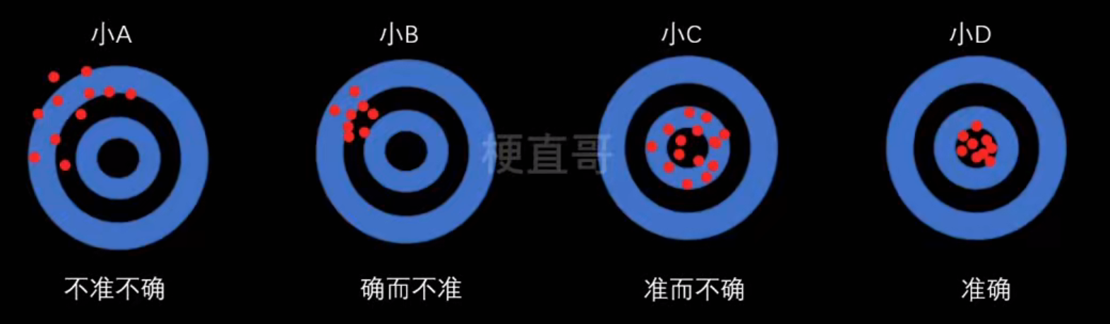
B的点比较集中,也就是比较确定
偏差、方差和噪声
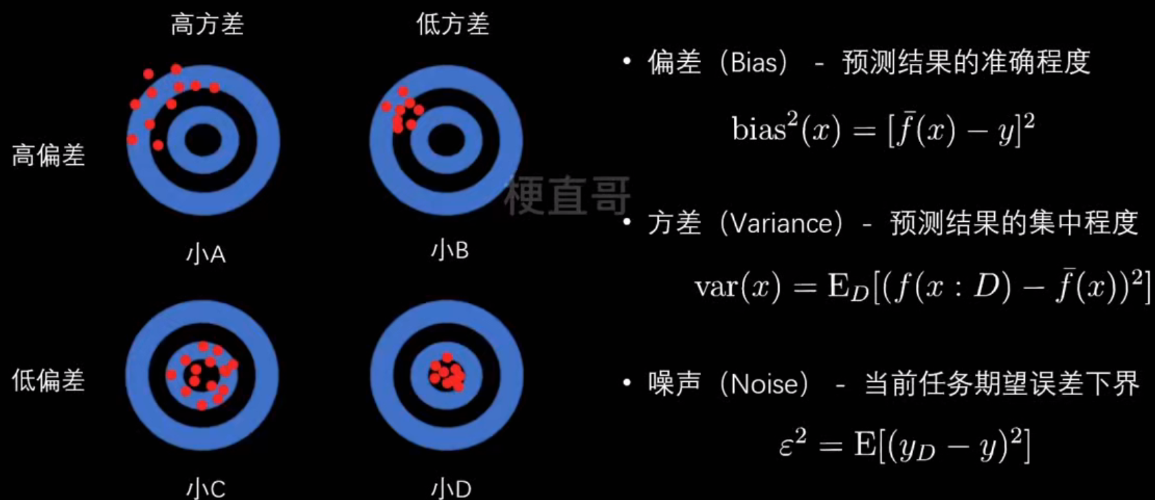
模型误差的组成:

- 高偏差的原因:模型本身不适合(线性模型拟合非线性数据);欠拟合(模型未收敛)
- 高方差的原因:模型过于复杂(特征太多);过拟合(噪声数据影响)
- 噪声难以避免的原因:观测误差,计算机精度误差,方法误差
偏差和方差的关系:
| 情况 | 偏差 | 方差 | 示意 |
|---|---|---|---|
| 高偏差、低方差 | 箭都集中在靶子一角(方向错,但很稳定) | ||
| 低偏差、高方差 | 箭散落在靶心周围(平均准,但不稳定) | ||
| 高偏差、高方差 | 箭乱飞,既不准又不稳 | ||
| 低偏差、低方差 | 箭都集中在靶心(理想模型) |
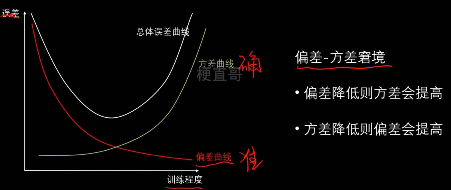
偏差、方差和模型复杂度的关系:
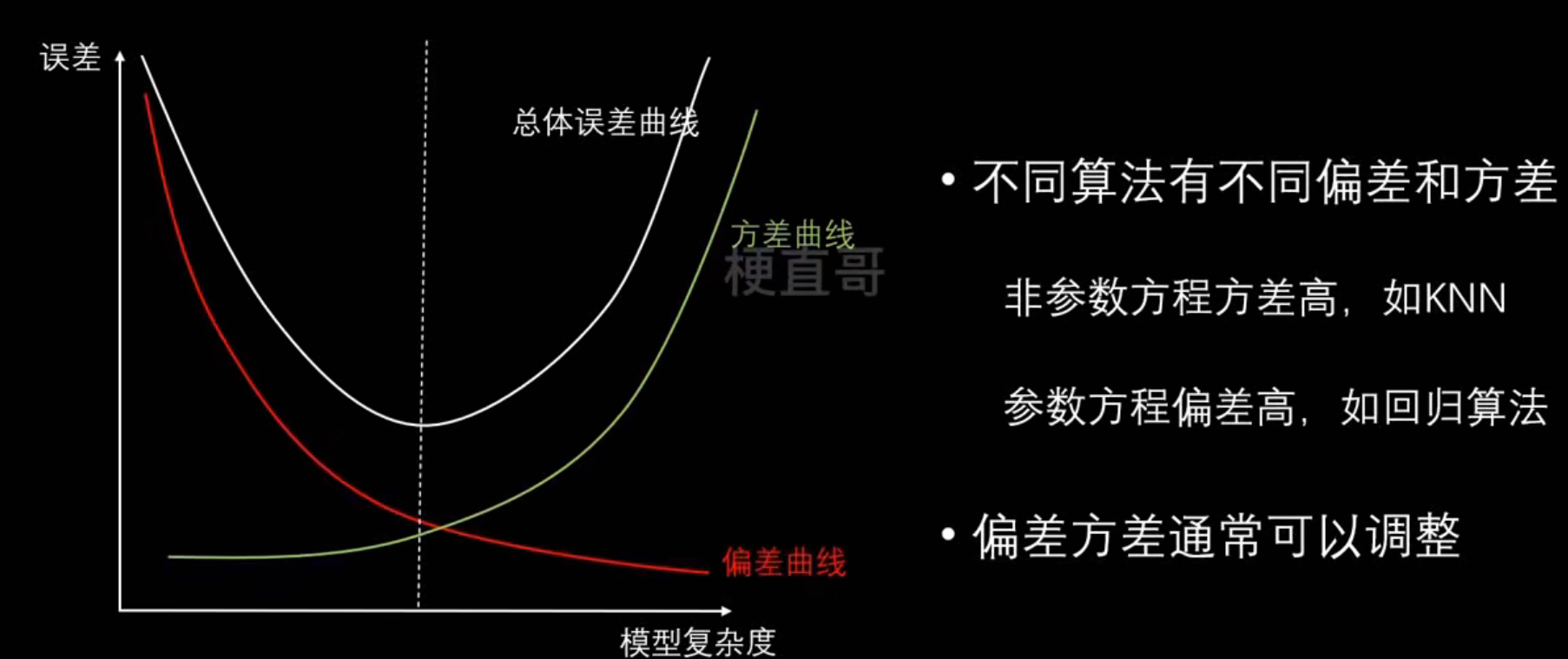
降低偏差:
- 寻找更好的特征
- 增加更多的特征
- 提高模型复杂度
降低方差:
- 尽量选低复杂度的模型
- 尽可能增加样本数
- 尽可能减少数据维度
- 使用验证集
- 使用正则化
正则化
本质上解决的是过拟合问题
在机器学习训练中,我们通常最小化一个**损失函数。**但是如果模型太复杂(比如参数太多、多层神经网络),它可能会“过度拟合训练集”,也就是把噪声也当成规律学了下来
为了防止这种情况,我们就给损失函数加一点“惩罚项”,不让模型的参数随便乱跑、变得太大。这就是 正则化
- 多项式逼近思想:
- 过拟合的真相:
如何尽量避免第三种情况呢?
控制高次项的系数
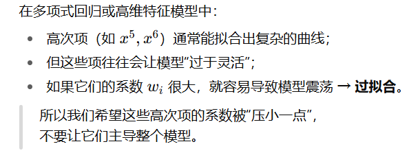
- 正则化
相似概念对比:
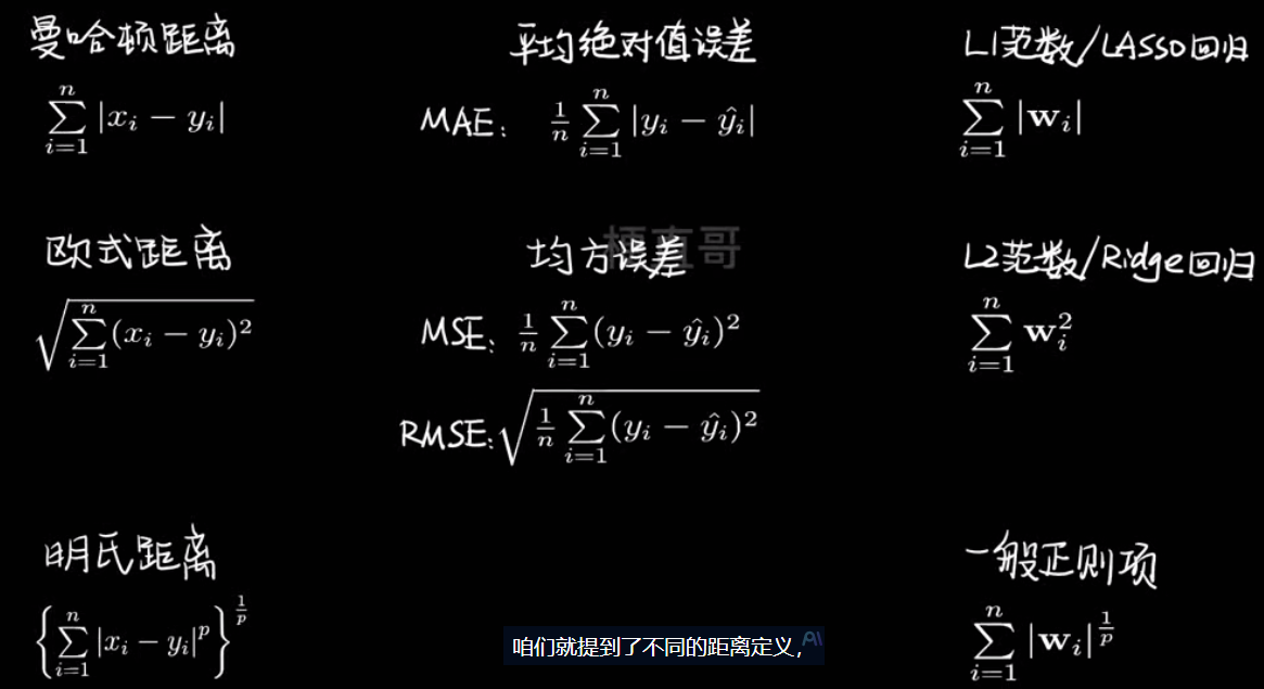
常见的两种正则化方法-----------LASSO回归和Ridge回归
模型泛化
泛化能力:
- 机器学习算法对于新鲜样本的适应能力
- 奥卡姆剃刀法则:能简单别复杂
- 泛化理论:衡量模型复杂度
如何知道自己的模型是否理想?
过拟合的应对策略:
- 降低模型复杂度
- 降低数据维度
- 降噪
- 增加样本数
- 使用验证集
- 正则化:
- L1:LASSOR回归
- L2:Ridge回归
- L1+L2:弹性网络
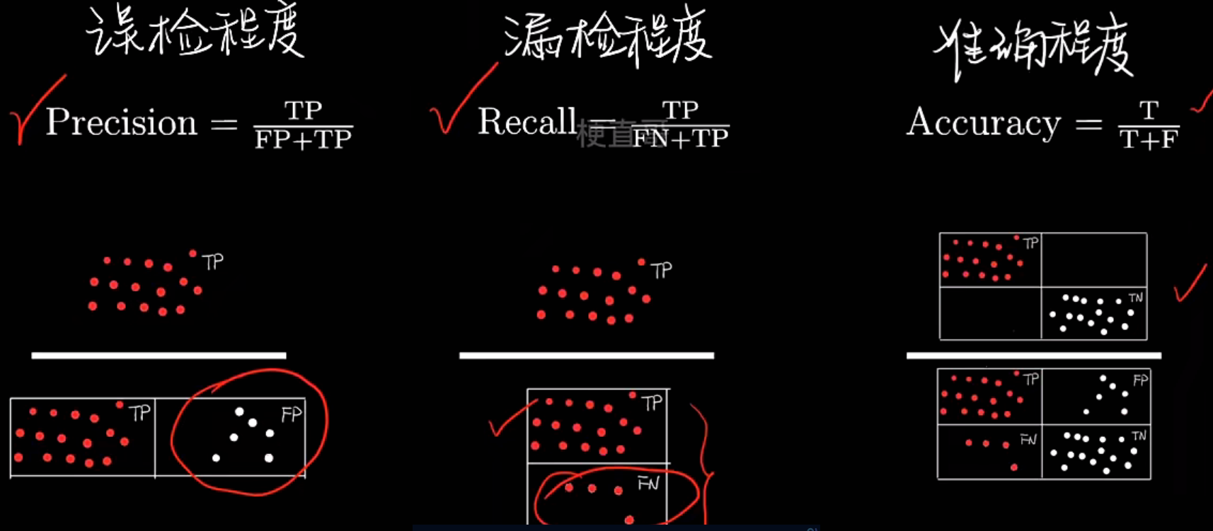
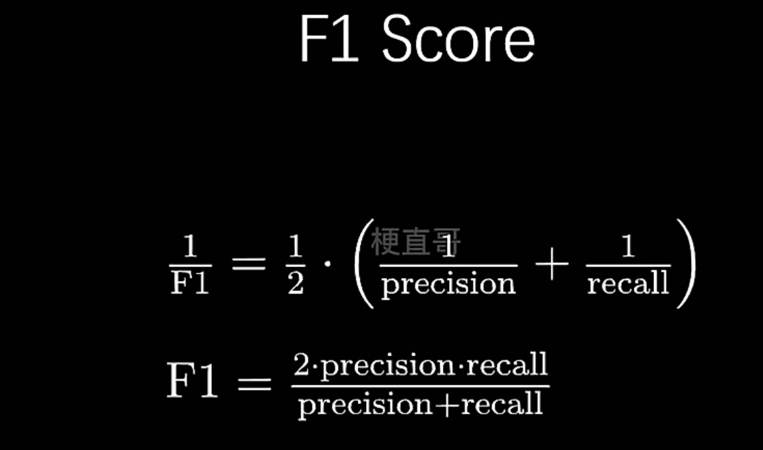
评价标准:混淆矩阵、精确率和召回率
Precision,Recall,F1 Score
- 混淆矩阵Confusion Matrix
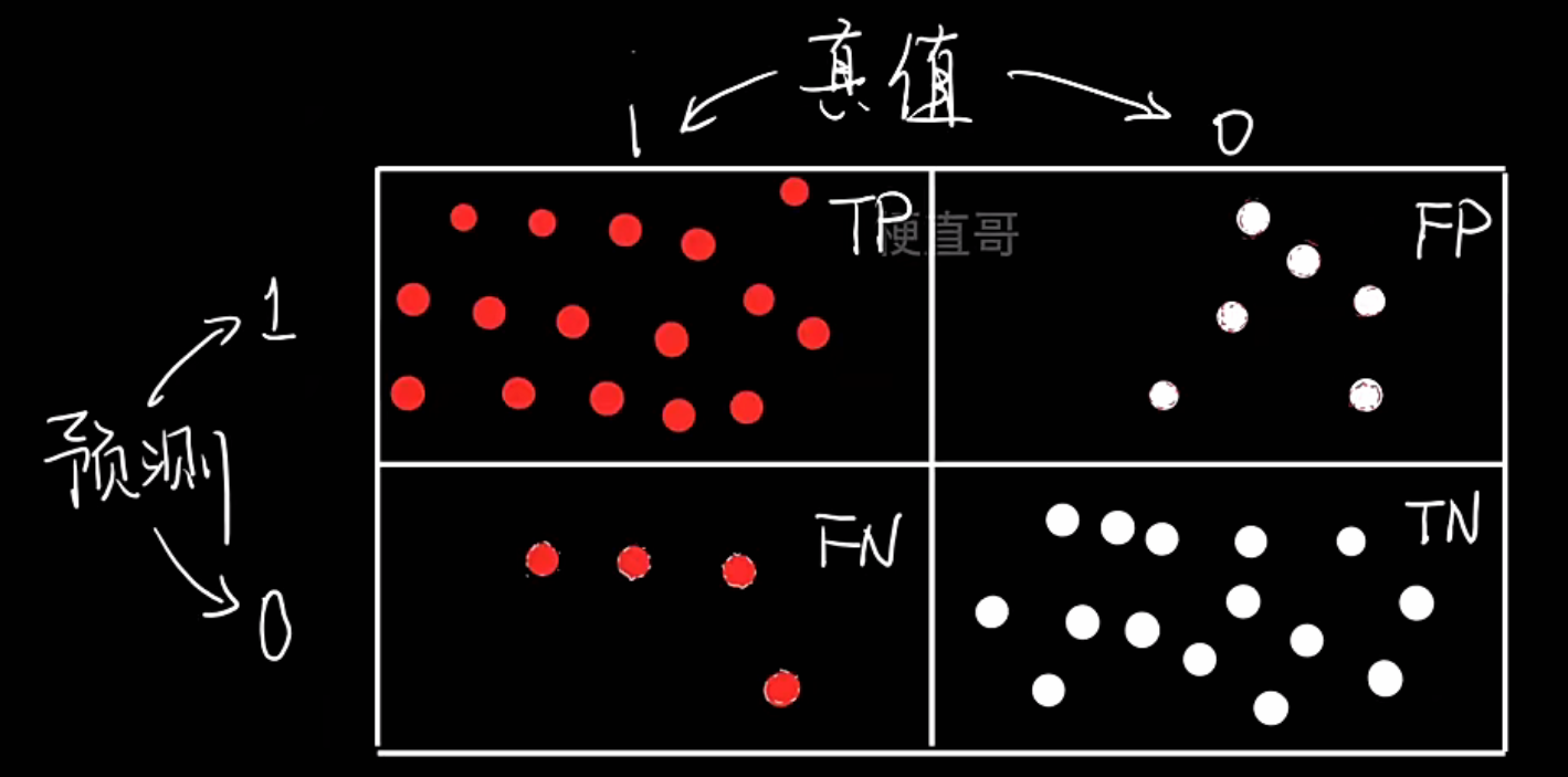
- 基于混淆矩阵的评价指标
| 指标 | 英文名 | 公式 | 含义 |
|---|---|---|---|
| 准确率 | Accuracy | (TP + TN) / (TP + FP + FN + TN) | 预测正确的总体比例 |
| 精确率 | Precision | TP / (TP + FP) | 预测为正的样本中,有多少是真的正 |
| 召回率 | Recall | TP / (TP + FN) | 所有真实正样本中,被模型识别出来的比例 |
| F1 值 | F1-Score | 2×(P×R)/(P+R) | Precision 与 Recall 的综合平衡 |
举个例子:
# 加载鸢尾花数据集
from sklearn import datasets
import numpy as npiris=datasets.load_iris()
X=iris.data
y=iris.target.copy()
y输出:
array([0, 0, 0, 0, 0, 0, 0, 0, 0, 0, 0, 0, 0, 0, 0, 0, 0, 0, 0, 0, 0, 0,0, 0, 0, 0, 0, 0, 0, 0, 0, 0, 0, 0, 0, 0, 0, 0, 0, 0, 0, 0, 0, 0,0, 0, 0, 0, 0, 0, 1, 1, 1, 1, 1, 1, 1, 1, 1, 1, 1, 1, 1, 1, 1, 1,1, 1, 1, 1, 1, 1, 1, 1, 1, 1, 1, 1, 1, 1, 1, 1, 1, 1, 1, 1, 1, 1,1, 1, 1, 1, 1, 1, 1, 1, 1, 1, 1, 1, 2, 2, 2, 2, 2, 2, 2, 2, 2, 2,2, 2, 2, 2, 2, 2, 2, 2, 2, 2, 2, 2, 2, 2, 2, 2, 2, 2, 2, 2, 2, 2,2, 2, 2, 2, 2, 2, 2, 2, 2, 2, 2, 2, 2, 2, 2, 2, 2, 2])
# 转化为二分类问题
y[y!=0]=1
y输出:
array([0, 0, 0, 0, 0, 0, 0, 0, 0, 0, 0, 0, 0, 0, 0, 0, 0, 0, 0, 0, 0, 0,0, 0, 0, 0, 0, 0, 0, 0, 0, 0, 0, 0, 0, 0, 0, 0, 0, 0, 0, 0, 0, 0,0, 0, 0, 0, 0, 0, 1, 1, 1, 1, 1, 1, 1, 1, 1, 1, 1, 1, 1, 1, 1, 1,1, 1, 1, 1, 1, 1, 1, 1, 1, 1, 1, 1, 1, 1, 1, 1, 1, 1, 1, 1, 1, 1,1, 1, 1, 1, 1, 1, 1, 1, 1, 1, 1, 1, 1, 1, 1, 1, 1, 1, 1, 1, 1, 1,1, 1, 1, 1, 1, 1, 1, 1, 1, 1, 1, 1, 1, 1, 1, 1, 1, 1, 1, 1, 1, 1,1, 1, 1, 1, 1, 1, 1, 1, 1, 1, 1, 1, 1, 1, 1, 1, 1, 1])
| 名称 | 英文全称 | 含义 | 模型预测结果 | 实际标签 | 是否预测正确 |
|---|---|---|---|---|---|
| TP | True Positive | 真正例 | 正 | 正 | ✅ |
| FP | False Positive | 假正例 | 正 | 负 | ❌ |
| FN | False Negative | 假负例 | 负 | 正 | ❌ |
| TN | True Negative | 真负例 | 负 | 负 | ✅ |
# 手动实现
from sklearn.model_selection import train_test_split
from sklearn.linear_model import LogisticRegressionX_train,X_test,y_train,y_test=train_test_split(X,y,random_state=666)logistic_regression=LogisticRegression()
logistic_regression.fit(X_train,y_train)
y_predict=logistic_regression.predict(X_test)TN=np.sum((y_predict==0)&(y_test==0))  #10
FP=np.sum((y_predict==1)&(y_test==0))  #0
FN=np.sum((y_predict==0)&(y_test==1))  #0
TP=np.sum((y_predict==1)&(y_test==1))  #28confusion_matrix=np.array([[TN,FP],[FN,TP]
])
confusion_matrix输出:
array([[10,  0],[ 0, 28]])
求精确率,召回率,F1
precision=TP/(TP+FP)  #1.0
recall=TP/(TP+FN)  #1.0
f1_score=2*precision*recall/(precision+recall) #1.0
# scikit-learn封装实现
from sklearn.metrics import confusion_matrixconfusion_matrix(y_test,y_predict)
输出:
array([[10,  0],[ 0, 28]])from sklearn.metrics import precision_score
from sklearn.metrics import recall_score
from sklearn.metrics import f1_scoreprecision_score(y_test,y_predict) #1.0
recall_score(y_test,y_predict)  #1.0
f1_score(y_test,y_predict)  #1.0
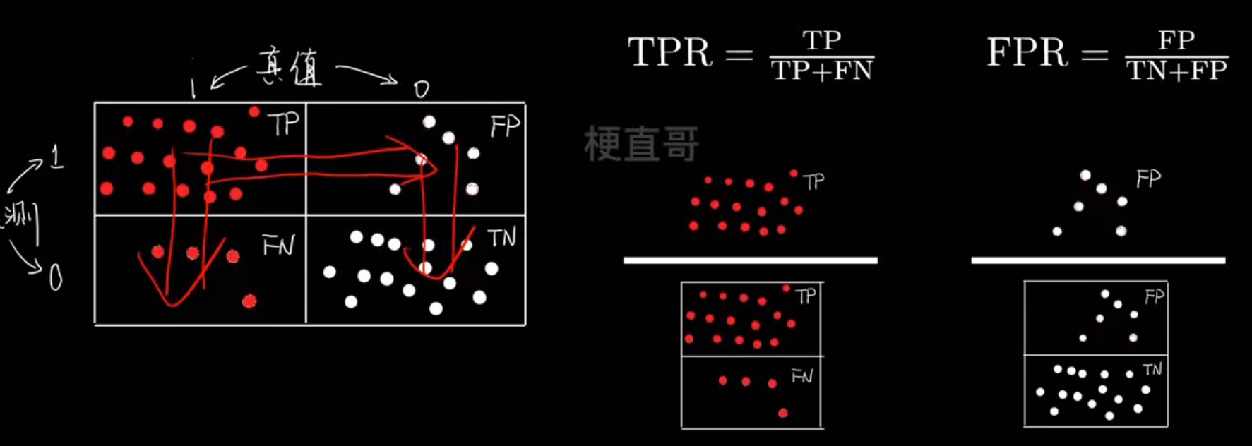
评价指标:ROC曲线
- ROC曲线
ROC 曲线(接收者操作特征曲线)是一个展示分类模型在不同阈值下性能表现的图,横轴是假阳性率(FPR),纵轴是真阳性率(TPR)
| 坐标 | 名称 | 公式 | 含义 |
|---|---|---|---|
| X 轴 | FPR(False Positive Rate) | FP / (FP + TN) | 实际为负却被误判为正的比例(误报率) |
| Y 轴 | TPR(True Positive Rate)= Recall | TP / (TP + FN) | 实际为正被正确识别出来的比例(召回率) |
- PR曲线
**PR 曲线(Precision–Recall Curve)**是在二分类问题中,用来评估模型性能的一种重要可视化方法。它展示了模型在不同阈值(threshold)下,Precision(查准率) 和 Recall(查全率) 之间的关系
| 对比项 | ROC 曲线 | PR 曲线 |
|---|---|---|
| 横轴 | FPR(假正率) | Recall(召回率) |
| 纵轴 | TPR(真正率) | Precision(精确率) |
| 衡量内容 | 模型整体区分能力(看模型能不能区分正负) | 模型在正类预测上的表现(看抓正类抓得多准、多全) |
| 是否受类别比例影响 | ❌ 不敏感 | ✅ 非常敏感 |
| 适用场景 | 正负样本数量接近时 | 正样本稀少时(类别极不平衡) |
| 典型任务 | 图像分类、性别识别 | 疾病检测、欺诈识别、垃圾邮件过滤 |
| 对应指标 | AUC(ROC) | AUC-PR |
| 曲线表现 | 对角线表示随机分类 | Precision 平均值接近正类比例表示随机分类 |
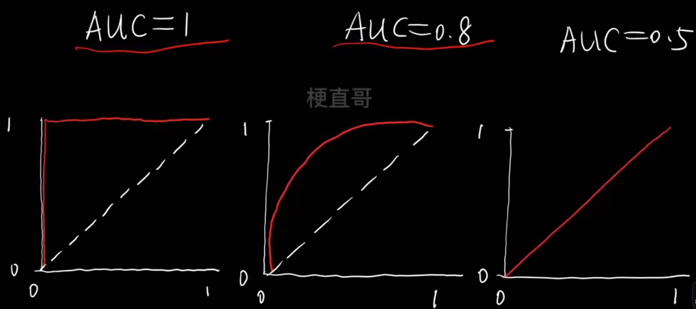
- AUC
AUC (Area Under the Curve) 就是 ROC 曲线下的面积,
用一个数值(0~1之间)来衡量模型的整体分类能力。
它表示:
随机取一个正样本和一个负样本,
模型把正样本排在负样本前面的概率。
AUC的判断标准:
举个例子:
前置准备:
import numpy as np
import matplotlib.pyplot as plt
from sklearn import datasetsiris = datasets.load_iris()
X = iris.data
y = iris.target.copy()# 转化为二分类问题
y[y!=0] = 1from sklearn.model_selection import train_test_split
from sklearn.linear_model import LogisticRegressionX_train, X_test, y_train, y_test = train_test_split(X, y, random_state=666)logistic_regression = LogisticRegression()
logistic_regression.fit(X_train,y_train)
y_predict = logistic_regression.predict(X_test)
y_predict输出:
array([1, 1, 1, 1, 0, 1, 1, 1, 1, 1, 1, 0, 0, 0, 1, 1, 0, 1, 1, 1, 1, 0,1, 0, 1, 1, 0, 1, 1, 1, 0, 0, 1, 1, 1, 1, 1, 1])
决策分数:
模型先给每个样本打一个分数,这个分数叫做“决策分数”(decision score);然后根据这个分数再决定——到底判为正类还是负类
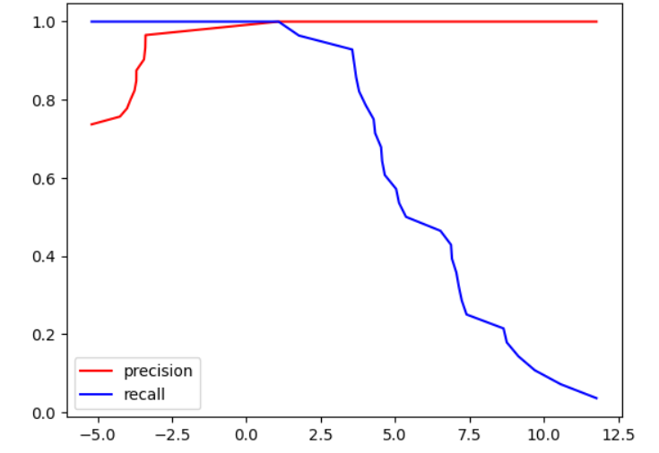
decision_scores = logistic_regression.decision_function(X_test)
decision_scores输出:
array([ 4.52818505,  6.87901472,  1.76728414,  6.52488998, -3.69893489,3.62555304,  4.5641345 ,  6.91106486,  5.03499692,  4.3292245 ,4.65382011, -3.43985382, -3.38750347, -3.39712028,  9.14590416,3.55830077, -5.19913952,  8.64478135,  7.05911342,  7.24100241,5.13254176, -3.758013  , 11.76868021, -3.89433573,  4.27903572,4.01351394, -4.2488403 ,  3.78927124,  8.75367646,  9.69578918,-4.01142913, -3.69538324,  3.69140718,  7.14170805,  1.08284202,5.36638089,  7.40154878, 10.56568001])
# 手写绘制 Precision–Recall vs Threshold 曲线
from sklearn.metrics import precision_score
from sklearn.metrics import recall_scoreprecision_scores = []
recall_scores = []
thresholds = np.sort(decision_scores)
for threshold in thresholds:# 大于阈值分为1,小于阈值分为0y_predict = np.array(decision_scores>=threshold,dtype='int')precision = precision_score(y_test,y_predict)recall = recall_score(y_test,y_predict)precision_scores.append(precision)recall_scores.append(recall)  plt.plot(thresholds, precision_scores, color='r',label="precision")
plt.plot(thresholds, recall_scores, color='b',label="recall")
plt.legend()
plt.show()
| 元素 | 含义 |
|---|---|
| 横轴(x-axis) | 决策阈值(threshold) = decision_function 的分界线 |
| 纵轴(y-axis) | Precision 或 Recall(介于 0 和 1 之间) |
| 红线(precision) | 查准率——预测为正的样本中有多少是真的正样本 |
| 蓝线(recall) | 查全率——所有真实正样本中被预测为正的比例 |
图形规律:
| 阈值变化方向 | Precision(红线) | Recall(蓝线) | 模型行为 |
|---|---|---|---|
| 阈值 ↓ | ↓ 降 | ↑ 升 | “激进”型:多报,查得全但误报多 |
| 阈值 ↑ | ↑ 升 | ↓ 降 | “保守”型:少报,查得准但漏报多 |
# Precision-Recall 曲线,简称PR曲线
plt.plot(recall_scores,precision_scores)
plt.xlabel("Recall")
plt.ylabel("Precision")
plt.show()
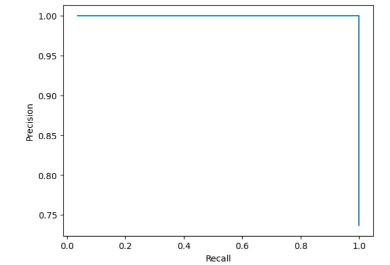
# scikit-learn中的PR曲线
from sklearn.metrics import precision_recall_curveprecision_scores, recall_scores,thresholds =  precision_recall_curve(y_test,decision_scores)plt.plot(thresholds, precision_scores[:-1], color='r',label="precision")
plt.plot(thresholds, recall_scores[:-1], color='b',label="recall")
plt.legend()
plt.show()
plt.plot(recall_scores,precision_scores)
plt.xlabel("Recall")
plt.ylabel("Precision")
plt.show()
# scikit-learn中的ROC曲线
from sklearn.metrics import roc_curvefpr, tpr, thresholds = roc_curve(y_test,decision_scores)
plt.plot(fpr,tpr)
plt.xlabel("FPR")
plt.ylabel("TPR")
plt.show()
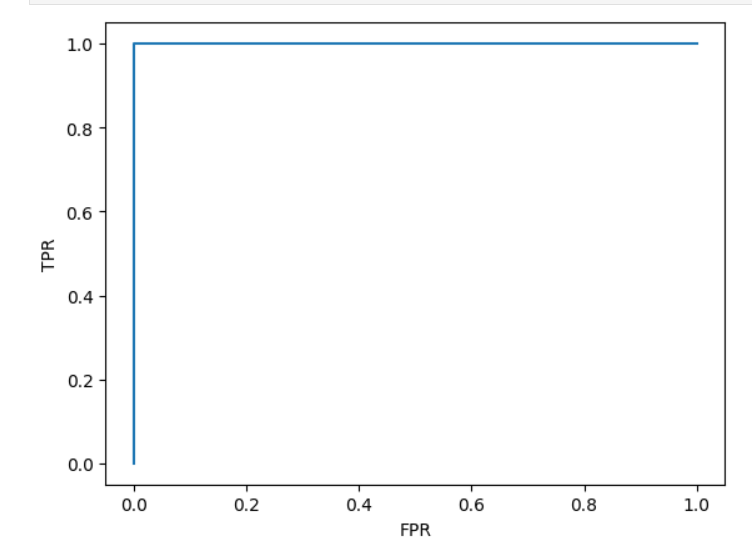
from sklearn.metrics import roc_auc_scoreauc = roc_auc_score(y_test,decision_scores)
auc输出:
np.float64(1.0)
4、决策树
树状决策:
- 假设数据中隐含树状特征结构
- 构建规则模型实现逼近
- 数据自上而下实现分类
决策树核心思想和原理
决策树的样子:
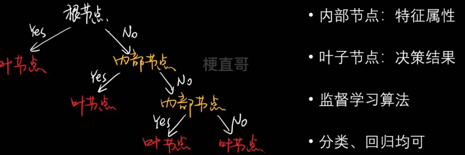
决策树的生成:

信息熵
- 信息熵
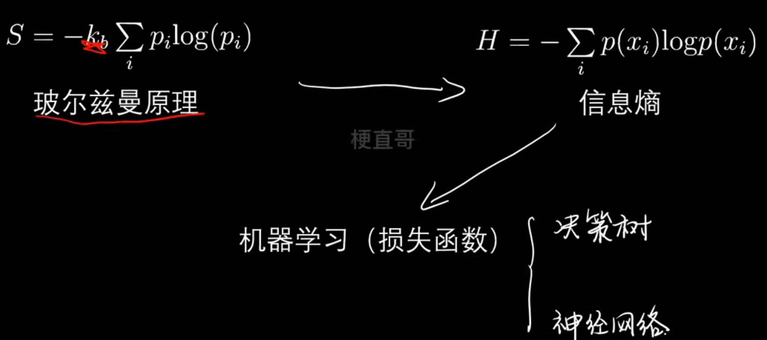
| 名称 | 含义 | 公式 | 应用场景 |
|---|---|---|---|
| 信息熵 (H§) | 度量系统自身的不确定性 | 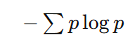 | 决策树分类(选择划分) |
| 交叉熵 (H(p,q)) | 度量两个分布差异 | 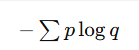 | 分类模型的损失函数 |
| MSE | 预测值与真实值的距离平方 | 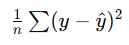 | 回归任务损失函数 |
- 各种熵
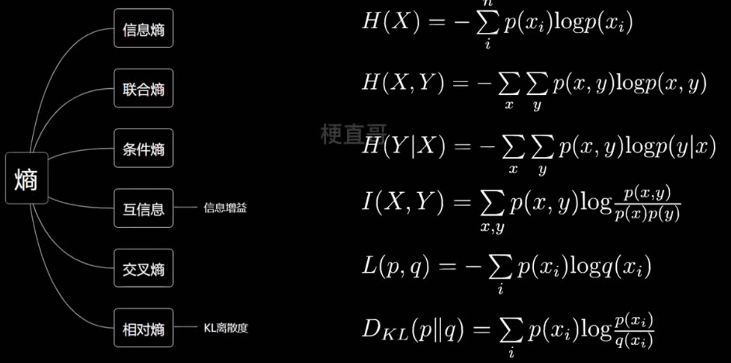
- 信息增益
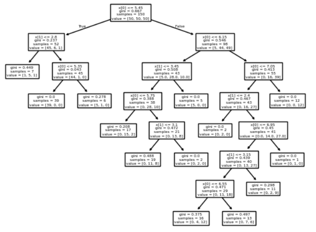
决策树分类任务和代码实现
# 二分类信息熵
import numpy as np
import matplotlib.pyplot as pltdef entropy(p):return -(p * np.log2(p) + (1 - p) * np.log2(1 - p))
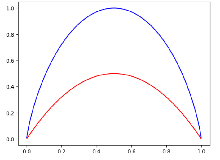
plot_x = np.linspace(0.001, 0.999, 100)
plt.plot(plot_x, entropy(plot_x))
plt.show()
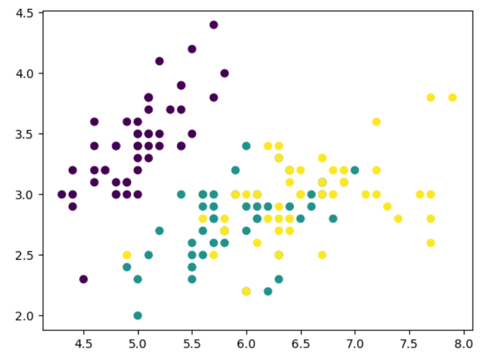
# 数据集
from sklearn.datasets import load_irisiris = load_iris()
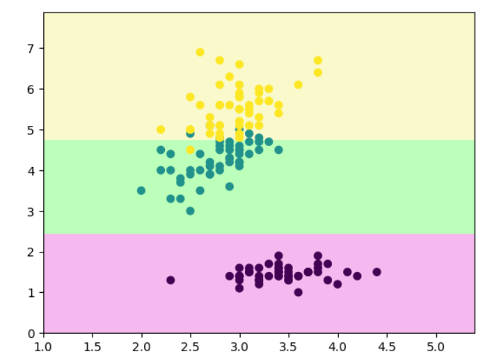
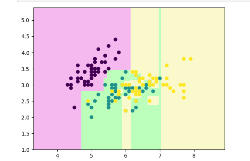
x = iris.data[:, 1:3]
y = iris.target
plt.scatter(x[:,0], x[:,1], c = y)
plt.show()
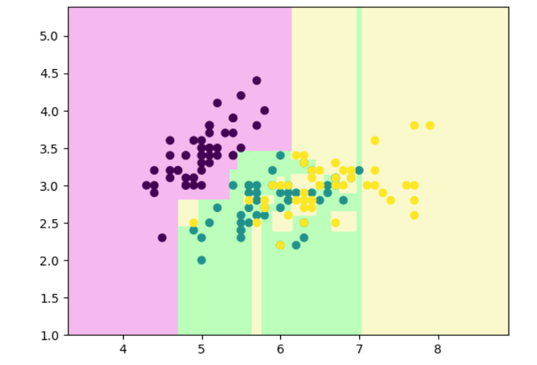
# 查看刚刚分类的效果
from sklearn.tree import DecisionTreeClassifier
clf = DecisionTreeClassifier(max_depth=2, criterion='entropy')
clf.fit(x, y)
def decision_boundary_plot(X, y, clf):axis_x1_min, axis_x1_max = X[:,0].min() - 1, X[:,0].max() + 1axis_x2_min, axis_x2_max = X[:,1].min() - 1, X[:,1].max() + 1x1, x2 = np.meshgrid( np.arange(axis_x1_min,axis_x1_max, 0.01) , np.arange(axis_x2_min,axis_x2_max, 0.01))z = clf.predict(np.c_[x1.ravel(),x2.ravel()])z = z.reshape(x1.shape)from matplotlib.colors import ListedColormapcustom_cmap = ListedColormap(['#F5B9EF','#BBFFBB','#F9F9CB'])plt.contourf(x1, x2, z, cmap=custom_cmap)plt.scatter(X[:,0], X[:,1], c=y)plt.show()decision_boundary_plot(x, y, clf)
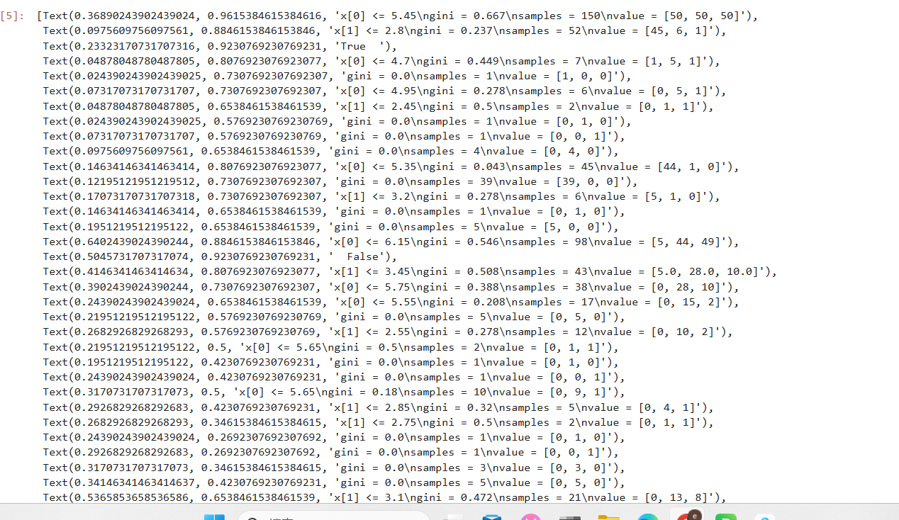
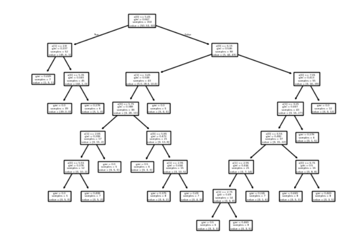
# sklearn中的决策树
from sklearn.tree import plot_tree
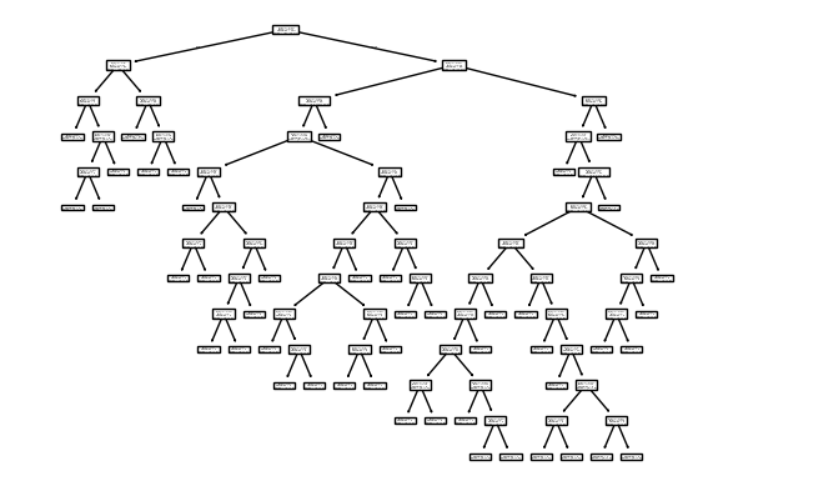
plot_tree(clf)
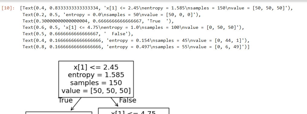
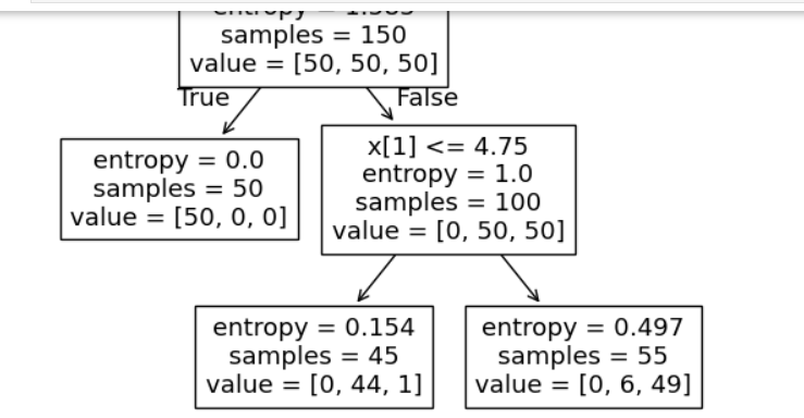
决策树的“最优划分条件”就是在每一步划分时,选择能让数据“最纯净”的特征和分割点
for 每个特征:for 每个候选划分点:→ 按阈值划分样本→ 计算左右熵→ 计算加权平均熵→ 若小于当前最小熵 → 更新最优划分# 最优划分条件
# 用 Python 的计数器统计每个类别在样本中出现的次数,得到每类样本数。
from collections import Counter
Counter(y) #Counter({np.int64(0): 50, np.int64(1): 50, np.int64(2): 50})
# 手写实现计算数据集的熵
def calc_entropy(y):counter = Counter(y)sum_ent = 0for i in counter:p = counter[i] / len(y)sum_ent += (-p * np.log2(p))return sum_ent
calc_entropy(y) #np.float64(1.584962500721156)def split_dataset(x, y, dim, value):index_left = (x[:, dim] <= value)index_right = (x[:, dim] > value)return x[index_left], y[index_left], x[index_right], y[index_right]
def find_best_split(x, y):best_dim = -1best_value = -1best_entropy = np.infbest_entropy_left, best_entropy_right = -1, -1for dim in range(x.shape[1]):sorted_index = np.argsort(x[:, dim])for i in range(x.shape[0] - 1):value_left, value_right = x[sorted_index[i], dim], x[sorted_index[i + 1], dim]if value_left != value_right:value = (value_left + value_right) / 2x_left, y_left, x_right, y_right = split_dataset(x, y, dim, value)entropy_left, entropy_right = calc_entropy(y_left), calc_entropy(y_right)entropy = (len(x_left) * entropy_left + len(x_right) * entropy_right) / x.shape[0]if entropy < best_entropy:best_dim = dimbest_value = valuebest_entropy = entropybest_entropy_left, best_entropy_right = entropy_left, entropy_rightreturn best_dim, best_value, best_entropy, best_entropy_left, best_entropy_right
find_best_split(x, y)
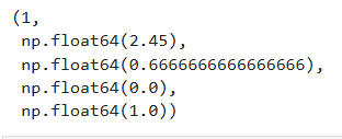
x_left, y_left, x_right, y_right = split_dataset(x, y, 1, 2.45)
find_best_split(x_right, y_right)
基尼系数
在分类问题中,我们希望每个节点(或样本集合)尽可能“纯”(pure),也就是样本尽量属于同一个类别。
基尼系数(Gini Impurity)就是用来衡量一个节点的不纯度的指标。
- 纯度高:节点中样本几乎都属于同一类 → 基尼系数小;
- 纯度低:节点中样本类别分布混乱 → 基尼系数大。
| 情形 | 类别分布 | 计算 | Gini值 | 解释 |
|---|---|---|---|---|
| 完全纯 | A类=100% | (1 - 1^2 = 0) | 0 | 最纯,节点完美 |
| 二分类均匀 | A=50%,B=50% | 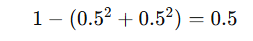 | 0.5 | 最不纯 |
| A=70%,B=30% | 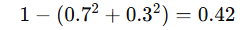 | 0.42 | 有一定纯度 |
应用----决策树在划分节点时,会遍历所有特征和可能的划分点,计算:
- 划分后的左右子节点的基尼系数;
- 计算加权平均基尼系数(即划分后的整体纯度);
- 选取加权基尼最小的划分作为最优划分
代码实现:
import numpy as np
import matplotlib.pyplot as pltdef entropy(p):return -(p * np.log2(p) + (1 - p) * np.log2(1 - p))
def gini(p):return 1 - p ** 2 - (1 - p) ** 2
plot_x = np.linspace(0.001, 0.999, 100)
plt.plot(plot_x, entropy(plot_x), color = 'blue')
plt.plot(plot_x, gini(plot_x), color = 'red')
plt.show()
基尼系数和信息熵
- 基尼系数运算稍快
- 物理意义略有不同
- 模型效果上差异不大
clf = DecisionTreeClassifier(max_depth=2, criterion='gini')
clf.fit(x, y)
注意!如果不指定,默认就是用基尼系数划分
决策树剪枝
为什么要剪枝?
- 目标:
- 降低复杂度,提高模型泛化能力
- 解决过拟合
- 手段:
- 限制深度(结点层数)
- 限制广度(叶子结点个数)
举个例子对比一下剪枝和不剪枝的区别:
不剪枝:
# 准备数据集
import numpy as np
import matplotlib.pyplot as plt
from sklearn.datasets import load_irisiris=load_iris()
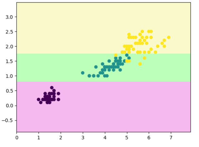
x=iris.data[:,0:2]
y=iris.targetplt.scatter(x[:,0],x[:,1],c=y)
plt.show()
# 使用决策树算法拟合样本数据
from sklearn.tree import DecisionTreeClassifierclf=DecisionTreeClassifier()
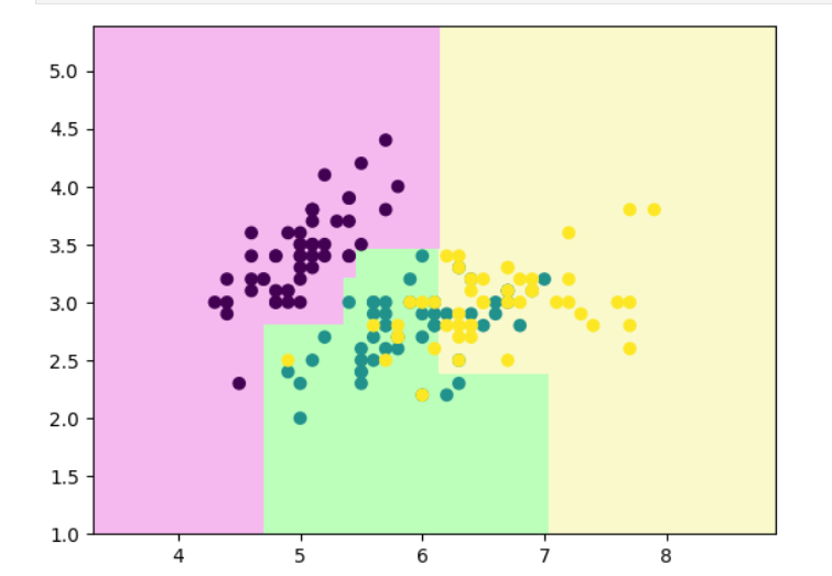
clf.fit(x,y)def decision_boundary_plot(X, y, clf):axis_x1_min, axis_x1_max = X[:,0].min() - 1, X[:,0].max() + 1axis_x2_min, axis_x2_max = X[:,1].min() - 1, X[:,1].max() + 1x1, x2 = np.meshgrid( np.arange(axis_x1_min,axis_x1_max, 0.01) , np.arange(axis_x2_min,axis_x2_max, 0.01))z = clf.predict(np.c_[x1.ravel(),x2.ravel()])z = z.reshape(x1.shape)from matplotlib.colors import ListedColormapcustom_cmap = ListedColormap(['#F5B9EF','#BBFFBB','#F9F9CB'])plt.contourf(x1, x2, z, cmap=custom_cmap)plt.scatter(X[:,0], X[:,1], c=y)plt.show()
# 绘制决策边界来查看绘制效果
decision_boundary_plot(x,y,clf)
# 绘制决策树样子
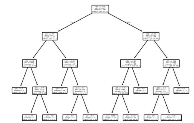
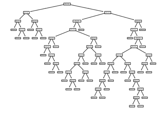
from sklearn.tree import plot_tree
plot_tree(clf)
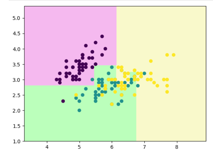
剪枝后:
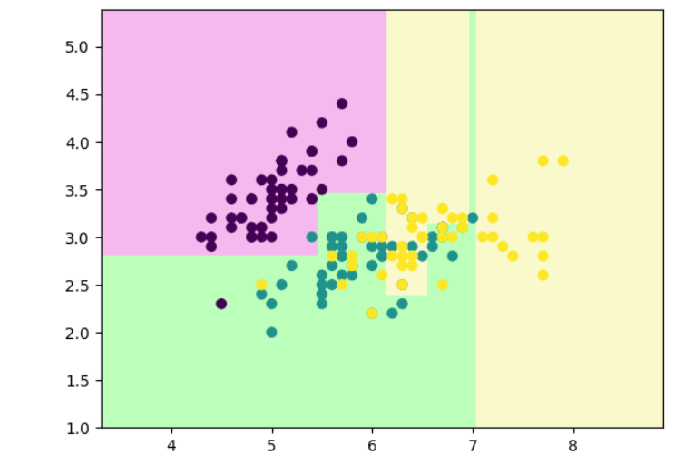
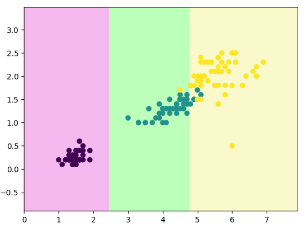
# 决策树剪枝
clf=DecisionTreeClassifier(max_depth=4)  #深度
clf.fit(x,y)
decision_boundary_plot(x,y,clf)
plot_tree(clf)
# 最小样本划分
clf=DecisionTreeClassifier(min_samples_split=20)
clf.fit(x,y)
decision_boundary_plot(x,y,clf)
plot_tree(clf)
# 最小节点样本数
# 即决策树的叶子节点数不能低于***,低于这个数就要向上合并
clf = DecisionTreeClassifier(min_samples_split=5)
clf.fit(x, y)
decision_boundary_plot(x, y, clf)
plot_tree(clf)
# 叶子节点样本的最小权重
# 此处是限制每个叶子节点的样本“权重占比”不能低于整个样本总权重的 3%
clf = DecisionTreeClassifier(min_weight_fraction_leaf=0.03)
clf.fit(x, y)
decision_boundary_plot(x, y, clf)
plot_tree(clf)
决策树回归任务代码实现
决策树如何回归?
由于相似的输入必然产生相似的输出
取节点平均值
| 项目 | 分类树(DecisionTreeClassifier) | 回归树(DecisionTreeRegressor) |
|---|---|---|
| 输出 | 类别(离散值) | 数值(连续值) |
| 划分指标 | 基尼系数 (Gini) 或 信息熵 (Entropy) | 均方误差 (MSE) 或 平均绝对误差 (MAE) |
| 叶节点值 | 投票最多的类别 | 样本目标值的平均数 |
| 应用场景 | 鸢尾花分类、垃圾邮件识别等 | 房价预测、温度估计、股票回归等 |
import warnings
warnings.filterwarnings('ignore')
import numpy as np
import matplotlib.pyplot as plt
from sklearn import datasets
from sklearn.model_selection import train_test_split, GridSearchCV
from sklearn.tree import DecisionTreeRegressor
from sklearn.metrics import r2_score# =========================
# 1) 数据集(改为加州房价)
# =========================
cal = datasets.fetch_california_housing()
x = cal.data
y = cal.target
# 把数据随机分为训练集与测试集(默认 75% 训练,25% 测试)
x_train, x_test, y_train, y_test = train_test_split(x, y, random_state=233)# =========================
# 2) 基础模型训练与评分
# =========================
reg = DecisionTreeRegressor()
reg.fit(x_train, y_train)# 返回 决定系数 R²
print(reg.score(x_test, y_test))
print(reg.score(x_train, y_train))输出:
0.5824658488130179
1.0
# =========================
# 3) 学习曲线(随训练样本数变化)
# =========================
plt.rcParams["figure.figsize"] = (12, 8)
max_depth = [2, 5, 10, 20]for i, depth in enumerate(max_depth):reg = DecisionTreeRegressor(max_depth=depth), reg = DecisionTreeRegressor(max_depth=depth)train_error = []test_error  = []for k in range(len(x_train)):reg.fit(x_train[:k+1], y_train[:k+1])y_train_pred = reg.predict(x_train[:k + 1])train_error.append(r2_score(y_train[:k + 1], y_train_pred))y_test_pred = reg.predict(x_test)test_error.append(r2_score(y_test, y_test_pred))plt.subplot(2, 2, i + 1)plt.ylim(0, 1.1)plt.title("Depth: {0}".format(depth))plt.plot([k + 1 for k in range(len(x_train))], train_error, label='train')plt.plot([k + 1 for k in range(len(x_train))], test_error,  label='test')plt.legend()plt.tight_layout()
plt.show()
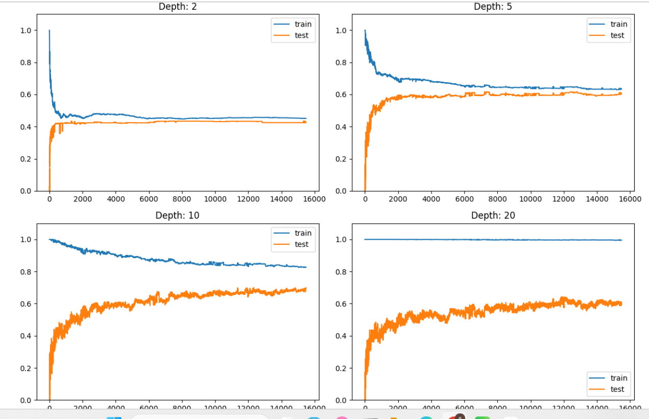
分析:
| 子图 | max_depth | 特征 | 模型表现解释 |
|---|---|---|---|
| 左上 | 2 | 训练和测试曲线都较平稳且收敛 | 模型较简单 → 偏差大、方差小,欠拟合。 |
| 右上 | 5 | 训练得分略高,测试得分上升后趋稳 | 模型复杂度适中 → 泛化较好。 |
| 左下 | 10 | 训练分数高,测试分数开始上升后停在0.6左右 | 模型开始过拟合。 |
| 右下 | 20 | 训练分数几乎为1.0,测试分数约0.6 | 模型完全记住训练数据 → 过拟合严重。 |
总体规律总结:
| 指标 | 随深度变化的趋势 |
|---|---|
| 训练集 R² | 随着深度增加而持续升高,趋近 1.0 |
| 测试集 R² | 先升后降,通常在中等深度(如 5~10)处达到最优 |
| 泛化能力 | 在 depth=5~10 时最好,过小欠拟合、过大过拟合 |
# =========================
# 4) 网格搜索,找到最佳的超参数
# =========================
params = {'max_depth': [n for n in range(2, 15)],'min_samples_leaf': [sn for sn in range(3, 20)],
}grid = GridSearchCV(estimator = DecisionTreeRegressor(),param_grid = params,n_jobs = -1
)grid.fit(x_train, y_train)print(grid.best_params_)
print(grid.best_score_)reg = grid.best_estimator_
print(reg.score(x_test, y_test))输出:
{'max_depth': 14, 'min_samples_leaf': 16}
0.7310066772774355
0.7284985242273161
分析:
- 最优超参
{'max_depth': 14, 'min_samples_leaf': 16}
含义:允许树最深到 14 层,但每个叶子至少要有 16 个样本。尽管深度看起来偏大,但配合较大的min_samples_leaf会强制合并小叶子、起到“平滑/正则化”的作用,从而抑制过拟合。这也解释了为什么之前max_depth=20会过拟合,而现在加了叶子最小样本数后能泛化得更稳。 - 交叉验证成绩(内部验证)
best_score_ = 0.7310
这是在训练集上做 K 折(默认 5 折)交叉验证得到的平均 R²。它代表你在看不见的折上(相当于验证集)的期望表现。 - 独立测试集成绩
reg.score(x_test, y_test) = 0.7285
与best_score_非常接近(0.731 vs 0.728),说明CV 评估与真正泛化误差吻合,配置稳定,没有明显的过拟合或数据泄漏。对加州房价这种噪声较多、非线性的回归问题来说,~0.73 的 R²已经是相当合理的树模型表现。
决策树优缺点和适用条件
- 优点
符合人类直观思维
可解释性强
能够处理数值型数据和分类型数据
能够处理多输出问题
- 缺点
容易产生过拟合
决策边界只能是水平或竖直方向
不稳定,数据的微小变化可能生成完全不同的树
举个例子:
# 正常情况下生成决策树
import numpy as np
import matplotlib.pyplot as plt
from sklearn.datasets import load_irisiris = load_iris()
X = iris.data[:,2:]
y = iris.targetfrom sklearn.tree import DecisionTreeClassifierdt_clf = DecisionTreeClassifier(max_depth = 2,random_state=666)
dt_clf.fit(X, y)def decision_boundary_plot(X, y, clf):axis_x1_min, axis_x1_max = X[:,0].min() - 1, X[:,0].max() + 1axis_x2_min, axis_x2_max = X[:,1].min() - 1, X[:,1].max() + 1x1, x2 = np.meshgrid( np.arange(axis_x1_min,axis_x1_max, 0.01) , np.arange(axis_x2_min,axis_x2_max, 0.01))z = clf.predict(np.c_[x1.ravel(),x2.ravel()])z = z.reshape(x1.shape)from matplotlib.colors import ListedColormapcustom_cmap = ListedColormap(['#F5B9EF','#BBFFBB','#F9F9CB'])plt.contourf(x1, x2, z, cmap=custom_cmap)plt.scatter(X[:,0], X[:,1], c=y)plt.show()decision_boundary_plot(X, y, dt_clf)
# 把第 131 个样本(X[130])的两个特征改成 [6, 0.5],然后重新训练模型。
X[130] = [6, 0.5]
dt_clf.fit(X, y)
decision_boundary_plot(X, y, dt_clf)
结果说明:
决策树对输入数据非常敏感(sensitive):
- 一点小的数据偏差、异常值、噪声都能改变划分结果;
- 深度越大,敏感性越强;
- 因此通常会配合参数控制(如
max_depth,min_samples_leaf,min_samples_split)或剪枝(ccp_alpha)防止过拟合。
5、神经网络
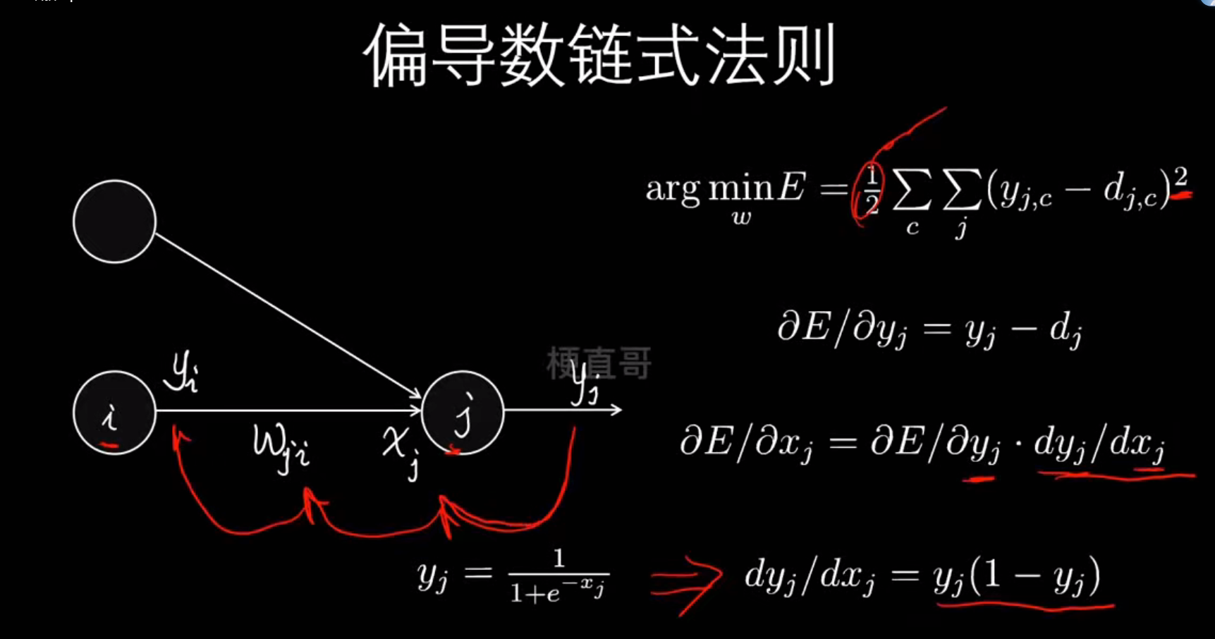
在神经网络中,每一次失败(预测错误)都会促进下一次成功(预测更准)——这正是“失败乃成功之母”的数学体现
| 俗语的含义 | 神经网络中的对应机制 |
|---|---|
| “失败” | 模型预测错误,损失函数(Loss)很大 |
| “从失败中学习” | 计算误差(Loss)并反向传播 |
| “吸取教训” | 调整权重(Weights)以减少错误 |
| “慢慢变得更好” | 不断迭代训练,Loss 越来越小 |
| “成功” | 模型收敛,预测准确率高 |
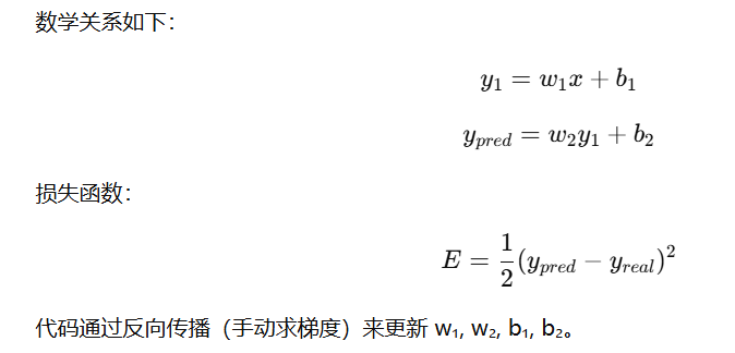
神经网络是什么?

倒过来发现就是多叉决策树

再换个角度理解:

神经网络核心思想和原理
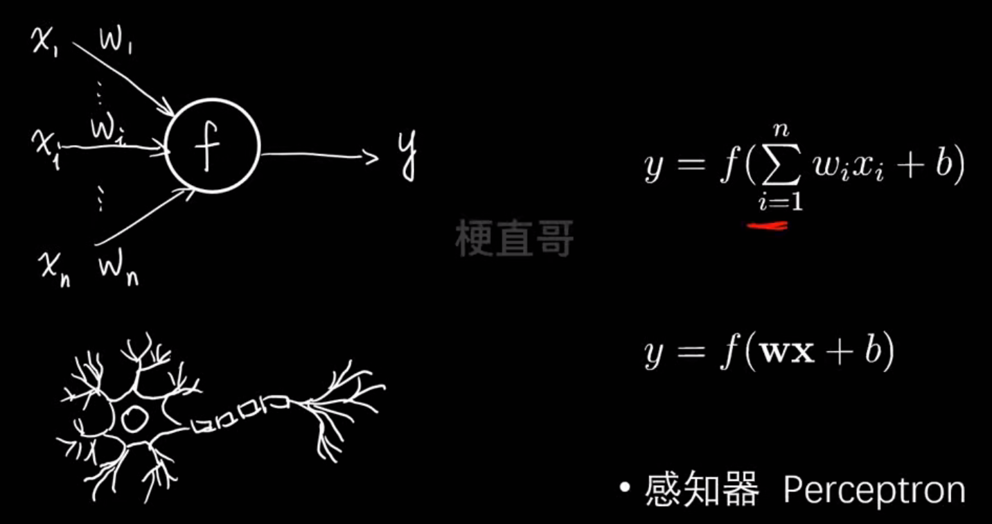
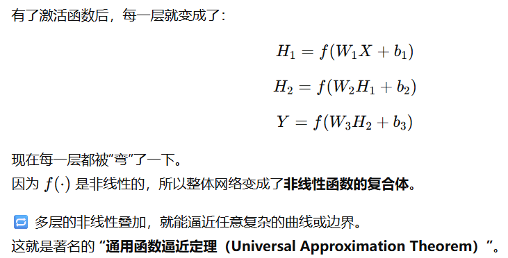
神经网络的核心思想是“用大量简单的线性单元,通过非线性组合,自动逼近复杂函数”。
也就是说:
- 每个神经元只会做一件简单的事:线性加权 + 非线性变换;
- 把很多神经元分层组合起来时,它就能表达非常复杂的模式(比如图像识别、语言理解、天气预测等)
这就是所谓的 “复杂性来自简单性”
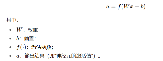
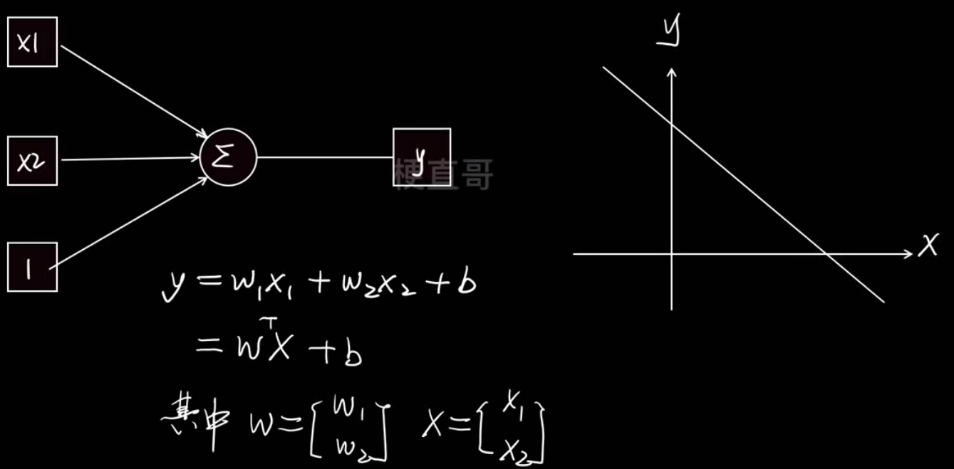
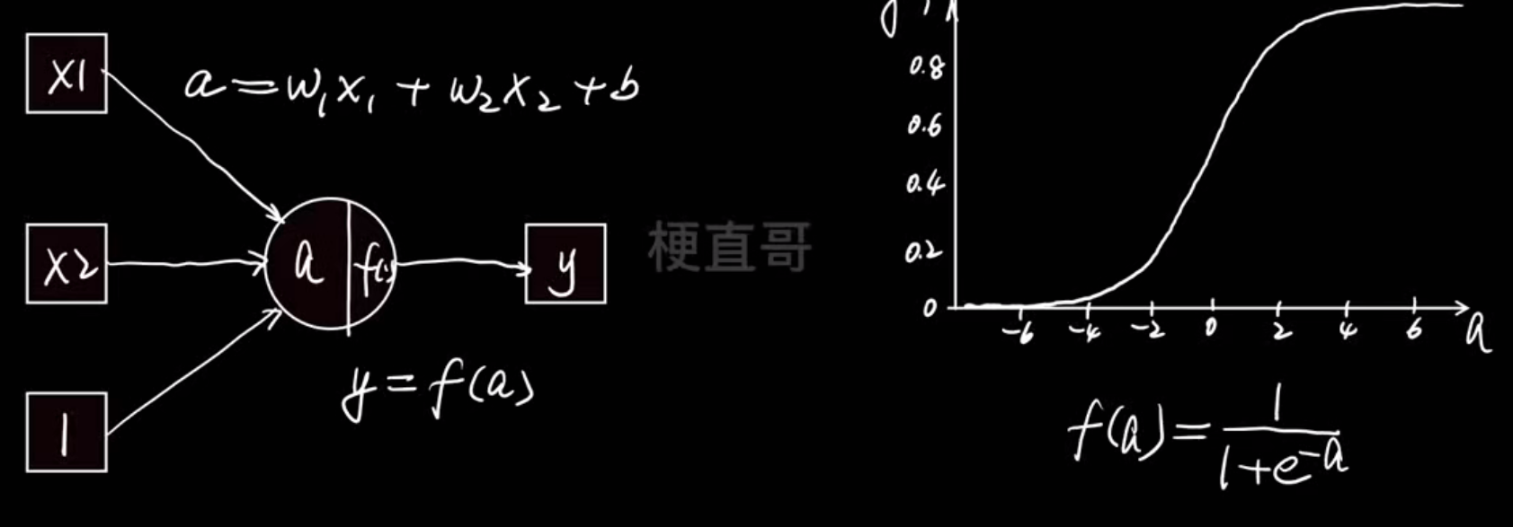
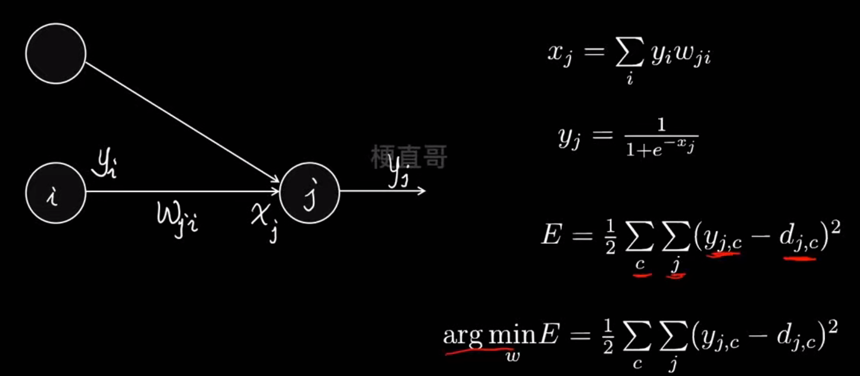
神经元模型:
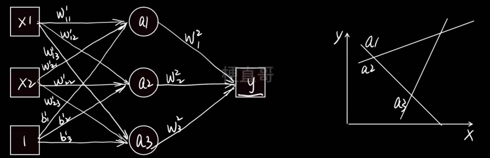
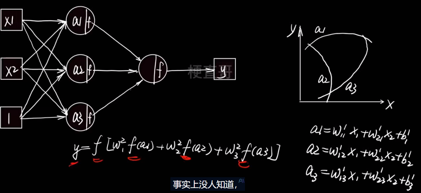
神经网络结构:

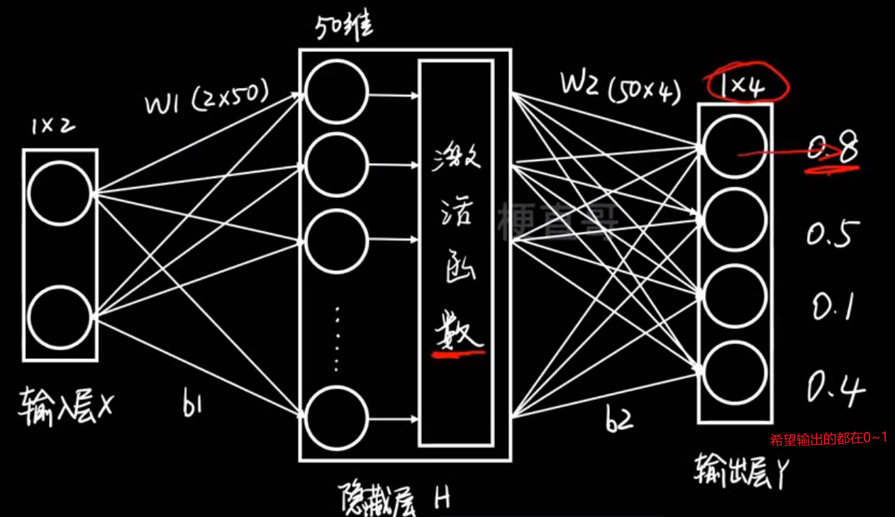
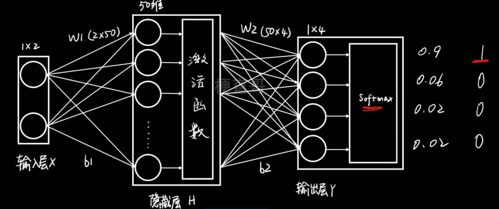
在这个例子中:
- 输入:2个特征(x₁, x₂)
- 经过隐藏层 50 个神经元的非线性组合
- 输出:4个结果(比如分类为A、B、C、D的概率)
也就是说,它在学习一个从二维特征 → 四维输出 的复杂非线性映射。
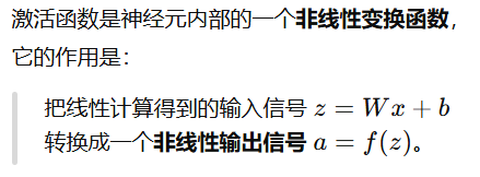
激活函数层:
本质就是把线性的变成非线性的
 有什么用:
有什么用:
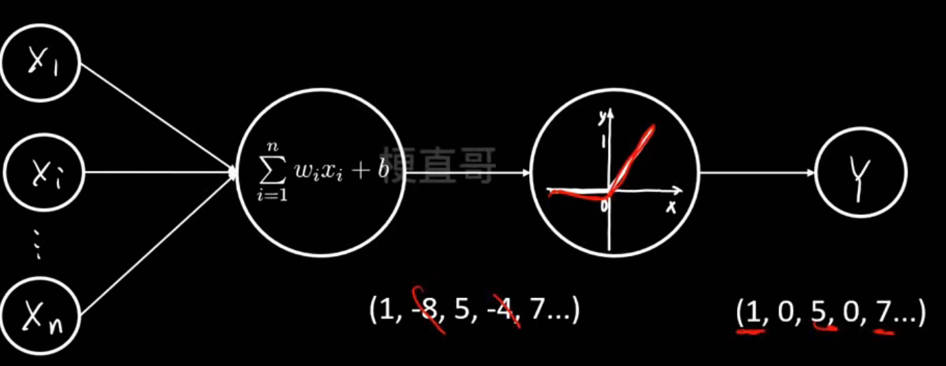
输出层:
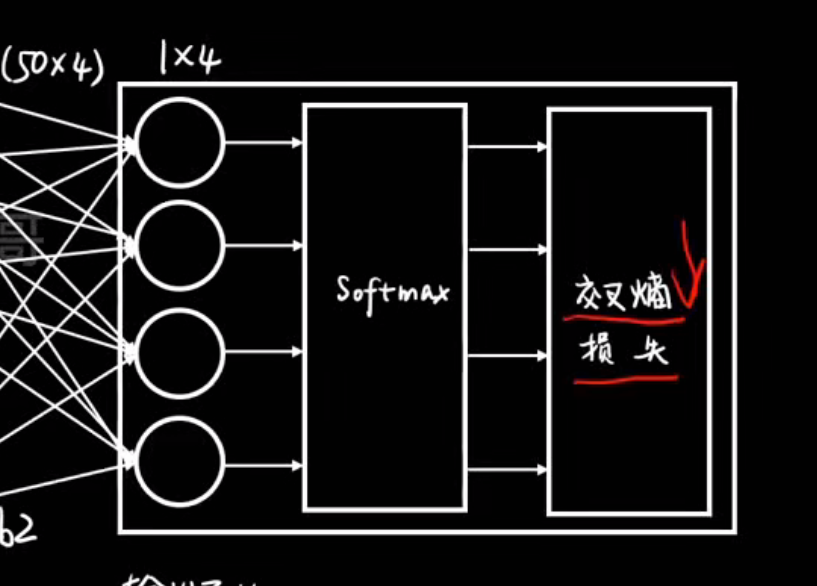
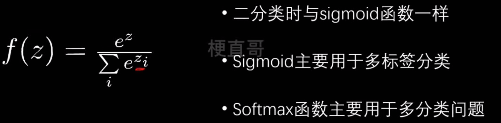
softmax层:
把一组任意实数(可以正、可以负)变换成一个概率分布
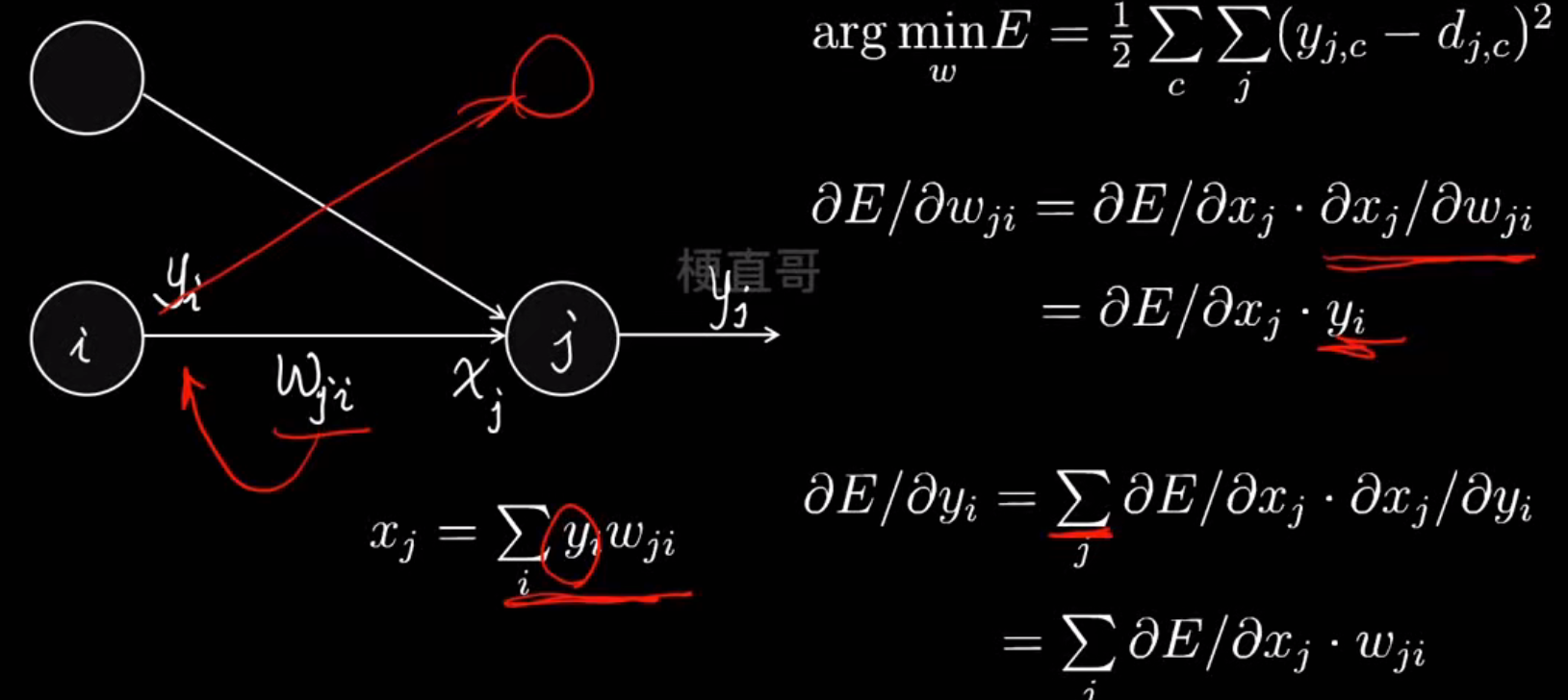
反向传播:
| 阶段 | 名称 | 方向 | 作用 |
|---|---|---|---|
| 1 | 前向传播 (Forward Propagation) | 从输入到输出 | 算出预测结果和损失 |
| 2 | 反向传播 (Backpropagation) | 从输出到输入 | 算出每个参数的“责任”,并更新它 |
- 计算损失对输出层每个权重的影响;
- 再计算损失对隐藏层权重的影响;
- 一层层往回传播“误差信号”。
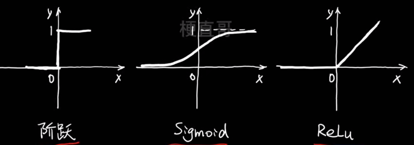
激活函数
为什么要使用激活函数?
右边的图非常关键:
- 横轴是输入 x,
- 纵轴是输出 y,
- 三条小曲线 a1,a2,a3是三组不同的线性组合(即三条直线)。
如果没有激活函数,这三条只是直线,无法表达复杂关系。
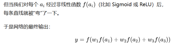
就成了多条非线性函数的加权叠加。
结果:这些“弯弯曲曲”的函数可以拼出任意复杂的形状(曲线、曲面、波动……)。这就是神经网络能拟合任意函数的关键
不管堆多少层,没有激活函数的网络永远只能画出直线,无法拟合曲线
最经典的sigmoid函数:
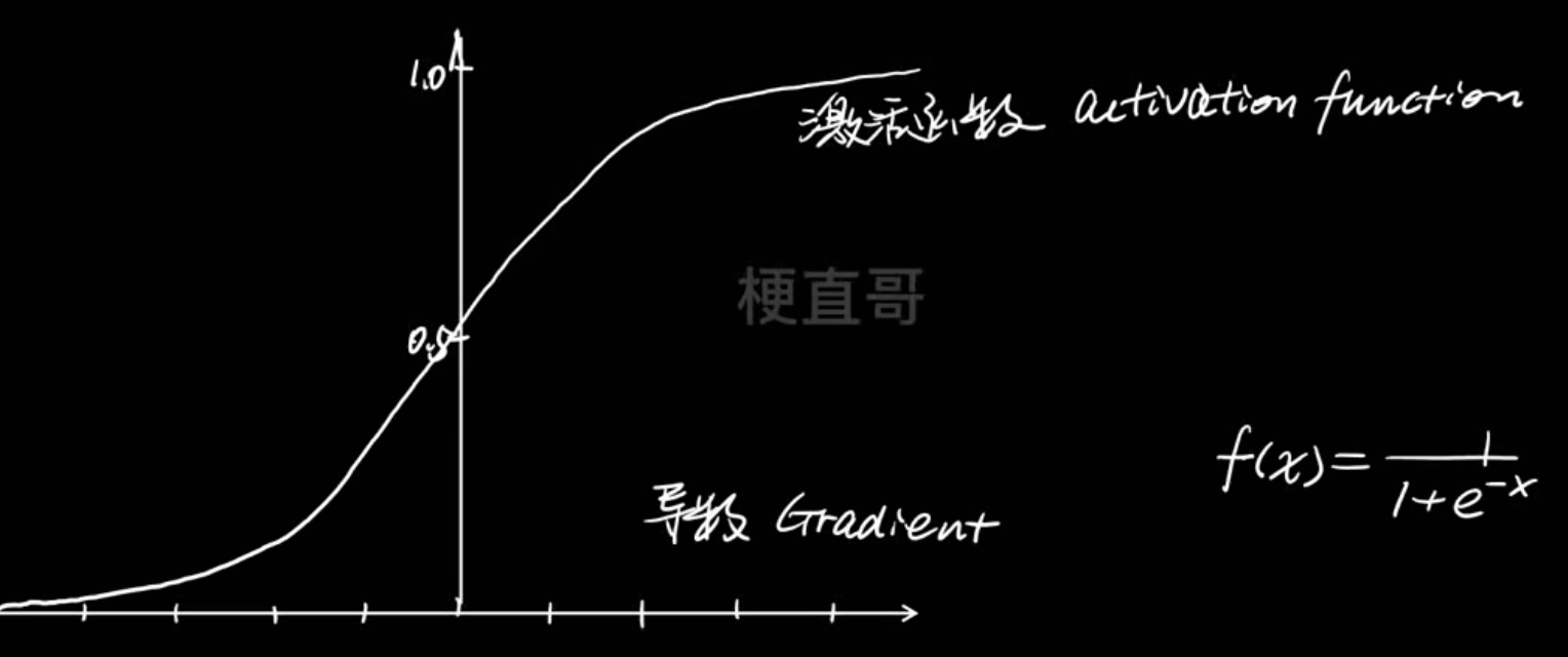
但这个函数会引起梯度消失的问题,且函数输出以0.5为中心而不是以0为中心,这会降低权重更新的效率
于是改进提出了Tanh函数---- 以 0 为中心,范围 (-1,1)
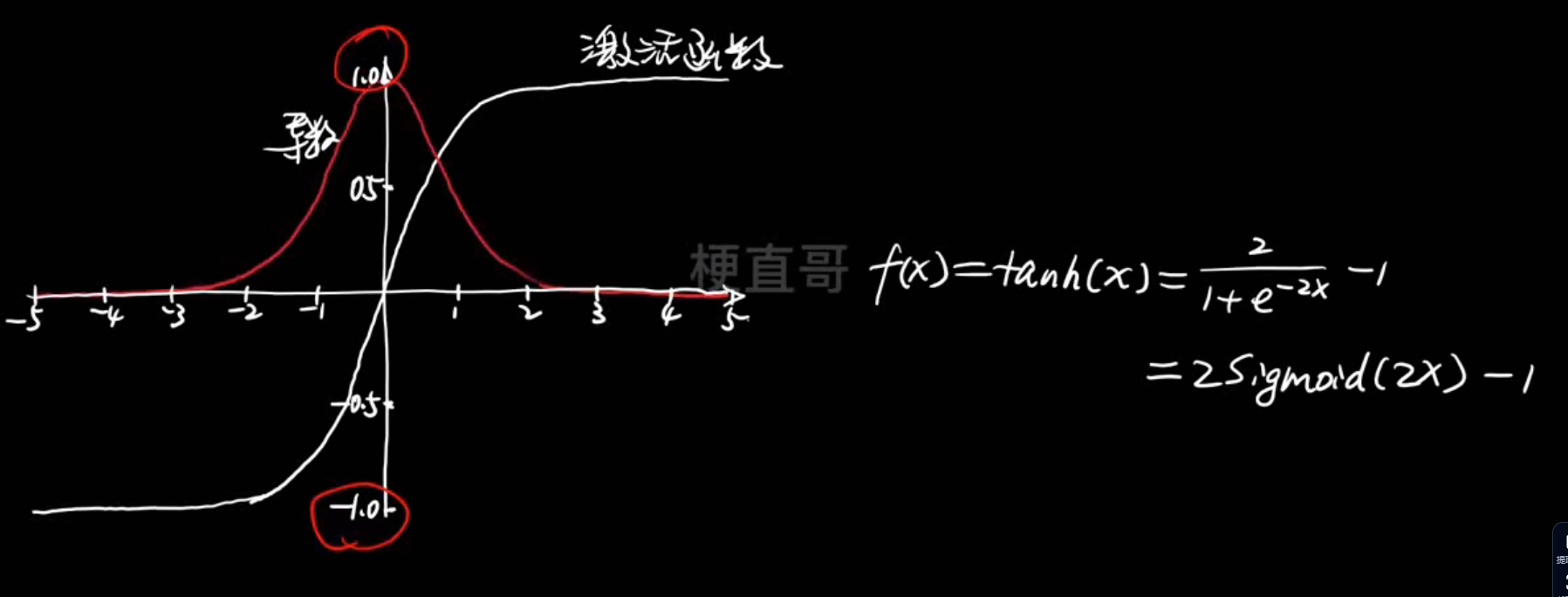
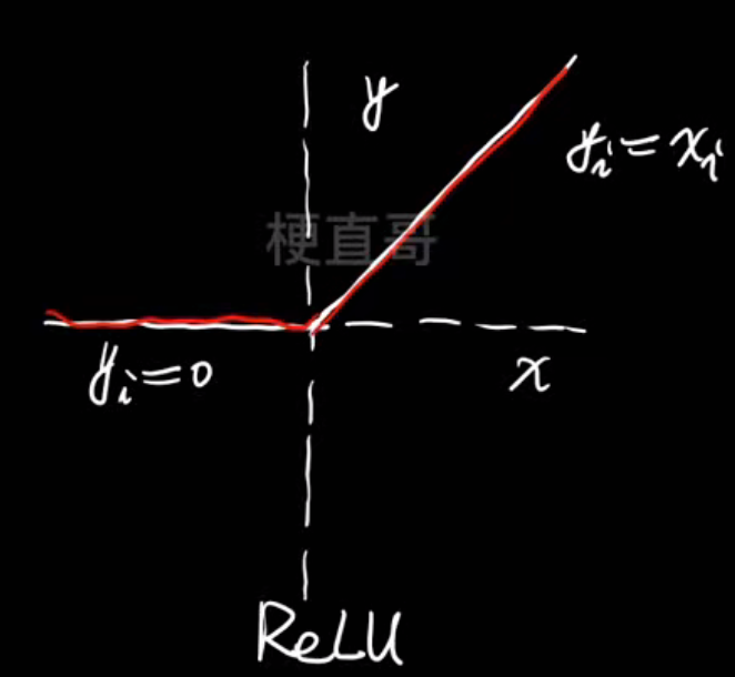
但是还是会有梯度消失,于是提出了 ReLU函数 ----- 线性区域梯度恒定,0~∞
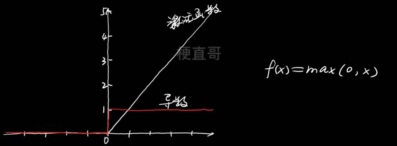
但是这个会导致神经元死亡问题,即输入为负的神经元的激活值总是为0
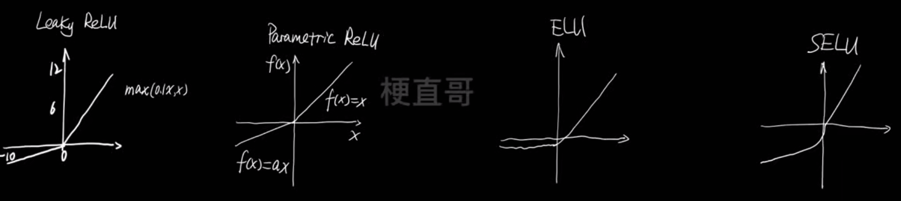
ReLU函数的各种变体:
还有一种经典的叫Softmax函数
如何选择激活函数?
- 不要把各种激活函数串联在一个网络使用
- 如果用ReLU,小心设置学习率
- 尽量不用sigmoid,可以试试tanh
正向传播与反向传播
模型学习的过程
- 正向传播(Forward)
输入数据从头到尾通过网络,产生预测结果。 - 计算损失(Loss)
计算预测结果和真实结果之间的差距。 - 反向传播(Backward)
计算每个参数对误差的“责任”,求出梯度。 - 参数更新(Gradient Descent)
根据梯度方向调整权重,减少下一次的错误。
┌────────────────────────────┐│ 正向传播:预测 → 计算损失 ││ 输入 x → 输出 ŷ → Loss L │└────────────────────────────┘↓┌────────────────────────────┐│ 反向传播:计算梯度 → 更新参数││ 误差反传 → 修正权重 W,b │└────────────────────────────┘
反向传播原理----最小化损失函数
梯度下降优化算法
优化原则:

搜索策略
- 批量梯度下降(Batch Gradient Descent)
原理:每次迭代使用 所有训练样本 来计算一次总体梯度:
特点:
- 精确方向:每次更新都沿着最陡的下降方向。
- 计算量大:需要遍历整个数据集才能更新一次。
- 内存开销大:难以在大规模数据上运行。
举例:
假如你有 10 万张图片,每次都要把 10 万张都过一遍再更新一次参数,非常慢。
适用场景:
- 小数据集
- 对精确收敛要求高的任务(如线性回归理论分析)
- 随机梯度下降(Stochastic Gradient Descent, SGD)
原理:每次只使用一个样本来计算梯度并更新参数:
特点:
- 更新频繁:几乎每看一个样本就更新一次。
- 速度快,但波动大:因为单个样本的梯度噪声大,损失曲线会“抖动”。
- 能跳出局部最优:噪声反而能帮助网络越过“局部坑”。
适用场景
- 在线学习(数据流式到达)
- 大数据集,快速粗略优化
- 深度学习早期探索阶段
- 小批量梯度下降(Mini-Batch Gradient Descent)
原理:每次使用一个小批量样本(mini-batch)(比如32或64个)计算平均梯度:
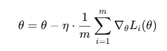
特点:
- 折中方案:兼顾稳定性和效率
- 计算并行化:适合GPU并行加速
- 波动适中:在梯度噪声和收敛稳定性之间取得平衡
- 是现代深度学习的默认选择
适用场景
- 几乎所有深度学习任务
- 大规模神经网络(CNN、Transformer等)
- 三者比较总结表
| 策略 | 每次使用样本数 | 更新频率 | 收敛速度 | 稳定性 | 是否支持GPU并行 | 应用场景 |
|---|---|---|---|---|---|---|
| 批量梯度下降 | 全部样本 | 低 | 慢 | 稳定 | 弱 | 小数据集,理论推导 |
| 随机梯度下降 | 1 个样本 | 高 | 快但震荡 | 不稳定 | 强 | 流式学习,大数据 |
| 小批量梯度下降 | 一小批(如32) | 中 | 快 | 稳定 | 强 | 主流深度学习训练 |
标配Adam算法
- 可视化理解(直观比喻)
假设你要从山顶下山到谷底:
- 批量下降:每次先测整个山的地形,一次走一步,稳但慢。
- 随机下降:闭着眼凭感觉走,每次只看脚下,快但容易乱走。
- 小批量下降:一小队人拿着局部地图,一边走一边修正方向,稳且高效。
步长选择
步长就是下降速度,大小要多次尝试,不能太大也不能太小
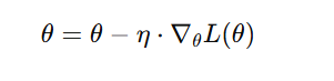
公式:
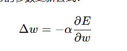
| 符号 | 含义 |
|---|---|
 | 参数更新量(每次权重要改多少) |
 | 学习率(learning rate,又叫“步长”) |
 | 误差函数对参数的偏导(梯度) |
 | 损失函数(Loss Function) |
梯度告诉我们“该往哪走”,而学习率 α 决定了“每一步走多远”。
- 如果 α 太大 → 一步跨太远,可能“越过山谷”,导致发散。
- 如果 α 太小 → 一步太短,收敛非常慢,甚至陷入局部震荡。
参数初始值的选择
初始值就是下山的起始点,初始值不同最小值也可能不同
多次尝试选择损失函数最小的
特征归一化
神经网络在训练时通过梯度下降更新参数
如果不同层的特征分布波动很大,模型会出现:
- 梯度爆炸 / 梯度消失
- 训练不稳定、收敛慢
- 激活函数进入饱和区(尤其是sigmoid/tanh)
归一化的目标是:保持每层输入和输出的分布稳定,让网络更快、更稳地学习
这在深层网络中尤为关键,因为层与层之间的信号传播容易“漂移”,即所谓的 Internal Covariate Shift(内部协变量偏移)
神经网络简单代码实现
| 符号 | 含义 |
|---|---|
| x | 输入 |
| w₁, b₁ | 第一层的权重、偏置 |
| y₁ | 第一层输出 |
| w₂, b₂ | 第二层的权重、偏置 |
| y₂(或ŷ, y_pred) | 网络预测输出 |
| y_real | 真实标签 |
| E | 损失(loss)或误差函数 |
简单神经网络—正向传播:
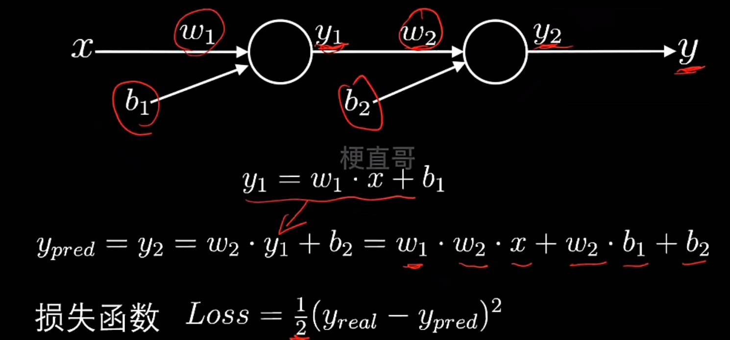
简单神经网络—反向传播:
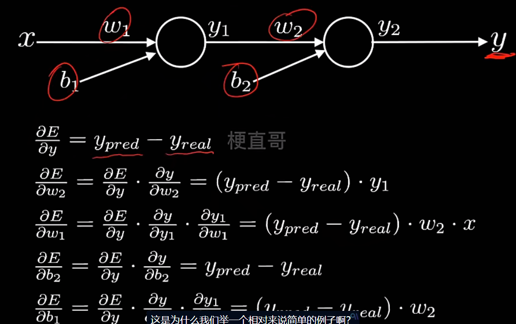
代码实现:
最简单的神经网络结构:
输入 x → 隐藏层 y1 → 输出层 y_pred
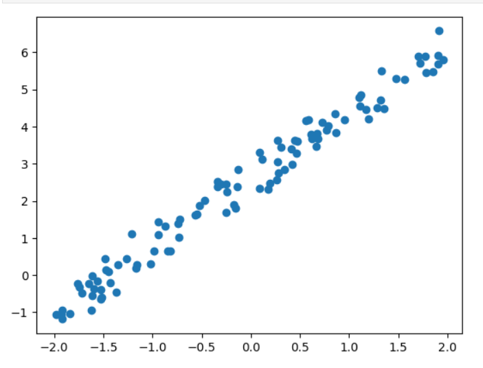
# 数据集
import numpy as np
import matplotlib.pyplot as pltw,b=1.8,2.5
np.random.seed(0)
x=np.random.rand(100)*4-2
noise=np.random.randn(100)/3
y=w*x+b+noisex=x.reshape(-1,1)
x.shape,y.shape输出:
((100, 1), (100,))
# 绘制图像
plt.scatter(x,y)
plt.show()
# sklearn中的神经网络
from sklearn.neural_network import MLPRegressor
reg= MLPRegressor(hidden_layer_sizes=(1,),  #带权重的输出层的权重activation='identity',   #不加激活函数learning_rate_init=0.01,  #初始学习率random_state=233
)
reg.fit(x,y)
reg.score(x,y)  #查看拟合效果输出:
0.974674992013746
y_pred=reg.predict(x)
plt.scatter(x,y)
plt.plot(x,y_pred,c='red')
plt.show()
# 查看权重和偏置
w1,w2=np.array(reg.coefs_).reshape(-1)
b1,b2=np.array(reg.intercepts_).reshape(-1)
print(w1,w2,b1,b2)输出:
-2.0230772887975506 -0.8994147672147477 0.20843202333485145 2.7673419504355397
# 结果就是前面定义的w=1.8,b=2.5,可能有一点偏差
w1 * w2, w2 * b1 + b2输出:
(np.float64(1.8195855887612917), np.float64(2.5798751106877256))
反向传播:
# 反向传播权重更新
# 生成4个符合标准正态分布 N(0,1) 的数
w1,w2,b1,b2=np.random.randn(4)
w1,w2,b1,b2
输出:
(np.float64(-0.35399391125348395),np.float64(-1.3749512934180188),np.float64(-0.6436184028328905),np.float64(-2.2234031522244266))y_real=y.reshape(-1,1)
lr=0.01
# 进行100次迭代训练,每次计算“前向传播 → 反向传播 → 参数更新”for i in range(100):y1 = w1 * x + b1y_pred = w2 * y1 + b2loss = ((y_real - y_pred) ** 2) / 2dy = y_pred - y_realdy1 = dy * w2dw1 = np.mean(x * dy1)dw2 = np.mean(y1 * dy)db1 = np.mean(dy1)db2 = np.mean(dy)w1 -= lr * dw1w2 -= lr * dw2b1 -= lr * db1b2 -= lr * db2print(w1, b1, w2, b2)输出:
-0.7865961506365119 -1.8052603505178628 -2.281516347579787 -1.5557865752893039
w1 * w2, w2 * b1 + b2输出:
(np.float64(1.7946319766205345), np.float64(2.562944426054817))
y_pred = w2 * (w1 * x + b1) + b2
plt.scatter(x, y)
plt.plot(x, y_pred, c = 'red')
plt.show()
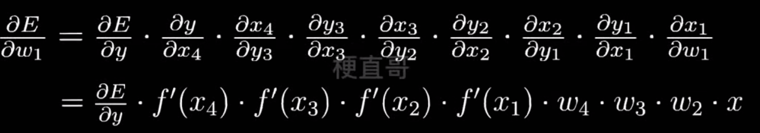
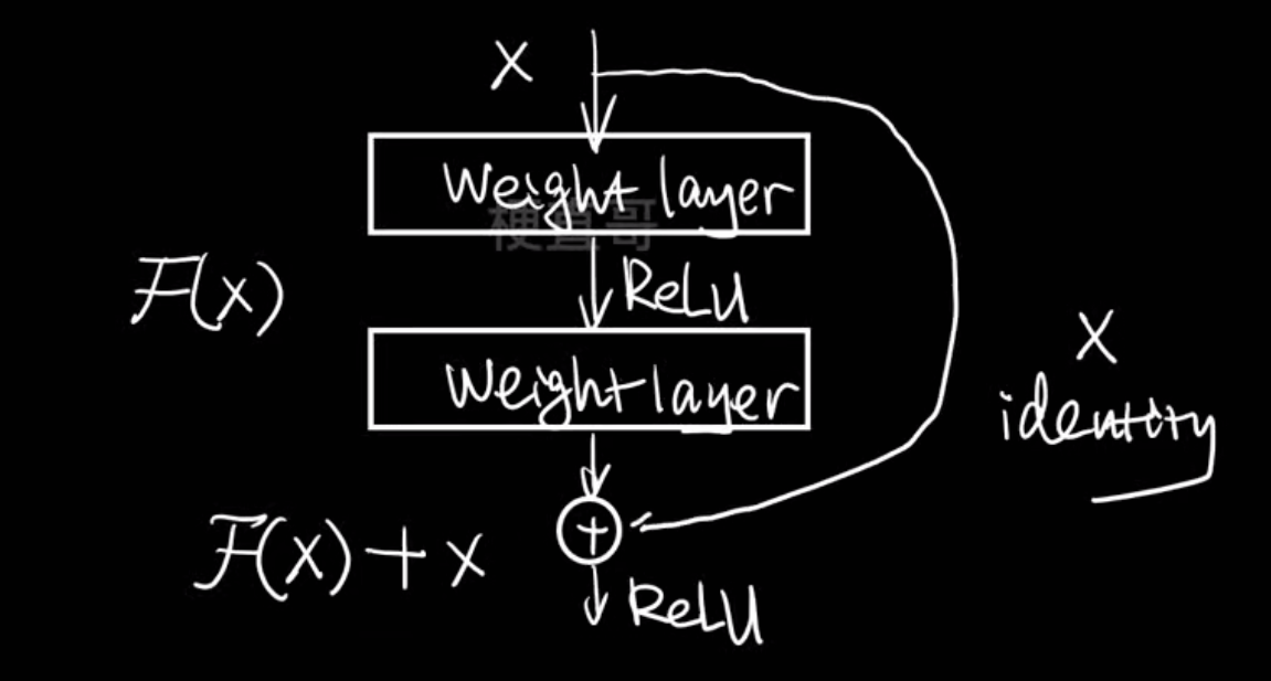
梯度消失和梯度爆炸
- 多层单神经元网络:
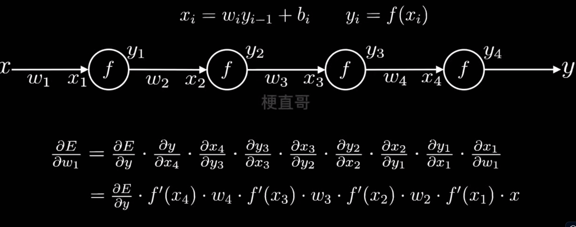
此网络有四个神经元串联四层:
x → [w₁,b₁,f] → y₁ → [w₂,b₂,f] → y₂ → [w₃,b₃,f] → y₃ → [w₄,b₄,f] → y₄ = ŷ
- 梯度消失:
梯度消失:深层网络中,梯度在反向传播时不断相乘变得越来越小,
导致前面的层几乎无法更新。原因:激活函数导数(比如Sigmoid)太小。
解决:换激活函数(ReLU)、加归一化、加残差
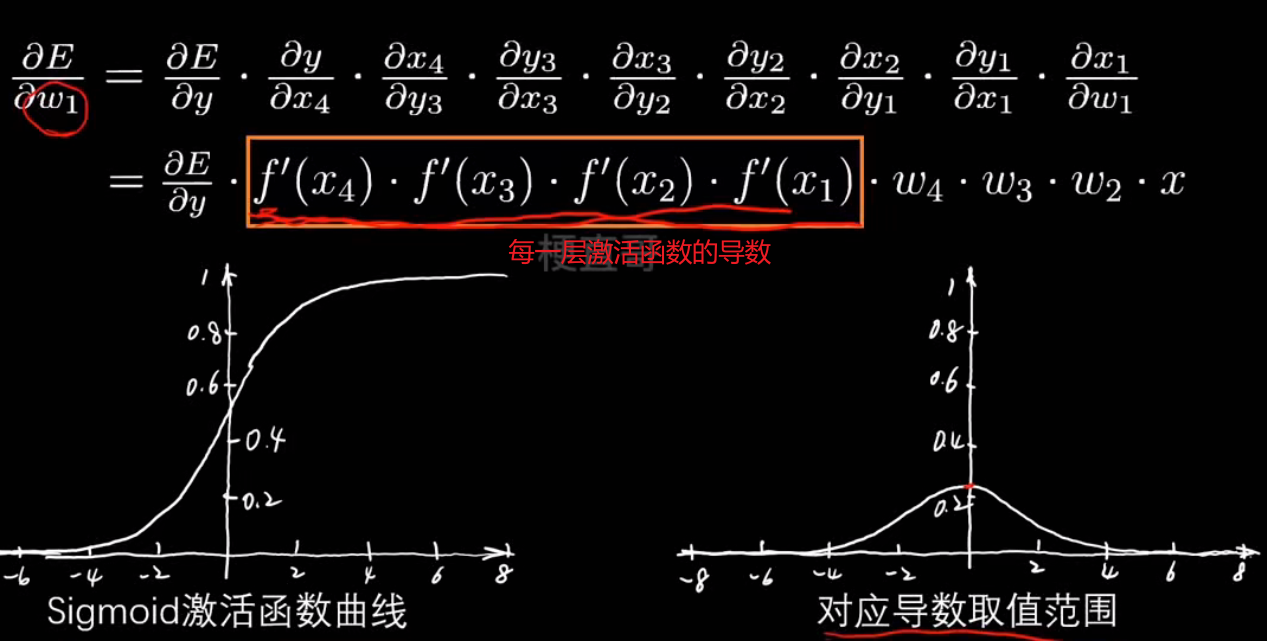
为什么叫梯度消失?
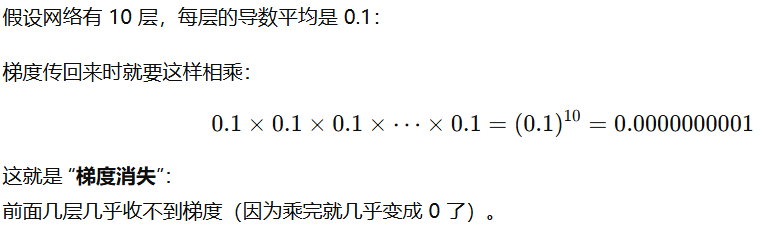
会导致网络退化
- 梯度爆炸
如果每一层的权重 wiw_iwi 或激活函数的导数 大于 1,这些数相乘后会迅速变得非常大——这就是梯度爆炸。
会导致网络不稳定
- 激活函数
更换更好的激活函数
梯度剪切(对梯度爆炸有用)

改进网络结构
模型选择
什么是模型选择?
在相同数据集上比较不同模型(KNN、决策树、逻辑回归)的性能
选择的原则:
- 模型效果
- 运算速度
- 算力要求
- 可解释性
代码实现:
# 不同模型的比较
import numpy as npfrom sklearn.neighbors import KNeighborsClassifierfrom sklearn.tree import DecisionTreeClassifierfrom sklearn.linear_model import LogisticRegression
from sklearn.preprocessing import PolynomialFeatures
from sklearn.pipeline import Pipeline
from sklearn.preprocessing import StandardScalerfrom sklearn.model_selection import cross_val_scoredef model_selection(x, y, cv):knn = KNeighborsClassifier(n_neighbors=3)dt = DecisionTreeClassifier(max_depth=5)lr = Pipeline([('poly', PolynomialFeatures(degree=2)),('log_reg', LogisticRegression(max_iter=500))])print('knn_score: %.4f, dt_score: %.4f, lr_score: %.4f' % (np.mean(cross_val_score(knn, x, y, cv=cv)),np.mean(cross_val_score(dt, x, y, cv=cv)),np.mean(cross_val_score(lr, x, y, cv=cv))))dataset = datasets.load_iris()
x = dataset.data
y = dataset.target
cv = 5
model_selection(x, y, cv)r输出:
knn_score: 0.9667, dt_score: 0.9533, lr_score: 0.9800
结果分析:
| 模型 | 平均准确率 | 解读 |
|---|---|---|
| KNN | 0.9667 | 高准确率,说明邻域投票效果好;Iris 是低维、类簇分明的数据,KNN表现优秀。 |
| 决策树 | 0.9533 | 稍低,可能因为 max_depth=5 限制了复杂度(过浅),或5折交叉验证中部分样本分界模糊。 |
| 逻辑回归(带二次项) | 0.9800 | 表现最佳。二次多项式让线性模型具备非线性拟合能力,同时泛化良好。 |
在Iris数据集上,逻辑回归(多项式特征) > KNN > 决策树。这与数据特性高度吻合 —— Iris 数据是近似线性可分的三分类问题
# 数据集从 Iris(鸢尾花) 换成了 Digits(手写数字识别)
dataset = datasets.load_digits()
x = dataset.data
y = dataset.target
cv = 5
model_selection(x, y, cv)输出:
knn_score: 0.9666, dt_score: 0.6328, lr_score: 0.9405
根据结果分析:
在手写数字识别任务中:
- KNN 表现最佳,因为“距离”能很好反映数字形状的相似性;
- 逻辑回归(二次特征) 次之,泛化稳定;
- 决策树(max_depth=5) 太浅,欠拟合严重;
调整决策树深度或引入更复杂模型(如随机森林、神经网络)后,准确率能轻松突破 0.95
# 使用神经网络模型
from sklearn.neural_network import MLPClassifier
nn = MLPClassifier(hidden_layer_sizes = (1,), activation = 'identity', learning_rate_init = 0.01, random_state = 233
)
np.mean(cross_val_score(nn, x, y, cv = 5))输出:
np.float64(0.42405756731662014)
结果分析:
| 参数 | 含义 | 实际效果 |
|---|---|---|
hidden_layer_sizes=(1,) | 只有一层隐藏层,且只有 1个神经元 | 模型几乎没有非线性表示能力 |
activation='identity' | 线性激活 (f(x)=x) | 网络整体退化成一个线性模型(等价于线性回归/逻辑回归) |
learning_rate_init=0.01 | 学习率 | 还可以接受 |
random_state=233 | 固定随机种子 | 确保结果可复现 |
只有 1 个神经元 + 线性激活函数,实际上相当于一个线性回归模型。 所以效果不佳
神经网络的模型选择:
nn = MLPClassifier(hidden_layer_sizes = (5,), activation = 'identity', learning_rate_init = 0.01, random_state = 233
)
np.mean(cross_val_score(nn, x, y, cv = 5))
输出:
np.float64(0.8809300526152894)
nn = MLPClassifier(hidden_layer_sizes = (100,), activation = 'identity', learning_rate_init = 0.01, random_state = 233
)
np.mean(cross_val_score(nn, x, y, cv = 5))输出:
np.float64(0.9176539770968741)
nn = MLPClassifier(hidden_layer_sizes = (5,), activation = 'relu', learning_rate_init = 0.01, random_state = 233
)
np.mean(cross_val_score(nn, x, y, cv = 5))输出:
np.float64(0.3060631383472609)
nn = MLPClassifier(hidden_layer_sizes = (100,100), activation = 'relu', learning_rate_init = 0.01, random_state = 233
)
np.mean(cross_val_score(nn, x, y, cv = 5))输出:
np.float64(0.943237387805633)
nn = MLPClassifier(hidden_layer_sizes = (100,50,100), activation = 'relu', learning_rate_init = 0.01, random_state = 233,solver='sgd'
)
np.mean(cross_val_score(nn, x, y, cv = 5))输出:
np.float64(0.9443593314763232)
nn = MLPClassifier(hidden_layer_sizes = (100,50,100,100,50,100,100,50,100), activation = 'relu', learning_rate_init = 0.01, random_state = 233
)
np.mean(cross_val_score(nn, x, y, cv = 5))输出:
np.float64(0.8920628288455585)
| 网络结构 | 激活 | 学习率 | 优化器 | 准确率 | 问题 / 优点 |
|---|---|---|---|---|---|
| (5,), identity | 线性 | 0.01 | Adam | 0.88 | 欠拟合 |
| (100,), identity | 线性 | 0.01 | Adam | 0.92 | 接近线性上限 |
| (5,), relu | 非线性 | 0.01 | Adam | 0.31 | 不收敛 |
| (100,100), relu | 非线性 | 0.01 | Adam | 0.94 | 最佳区间 |
| (100,50,100), relu | 非线性 | 0.01 | SGD | 0.94 | 稳定泛化好 |
| (100,…多层), relu | 非线性 | 0.01 | Adam | 0.89 | 过深→梯度不稳 |
| (100,50,100)+Scaler+LR=0.001 | relu | 0.001 | Adam | ⭐0.97~0.98 | 最优配置 |
神经网络优缺点和使用条件
优点:
- 范围广
- 问题
- 数据类型
- 效果好
- 泛化能力强
- 容错能力强
- 性能好
- 并行计算
- GPU or TPU计算
缺点:
- 训练难度大
- 训练时间长
- 黑盒不可解释
适用条件:
- 数据规模庞大,人工提取特征困难
- 无需解释,只要结果
6、支持向量机

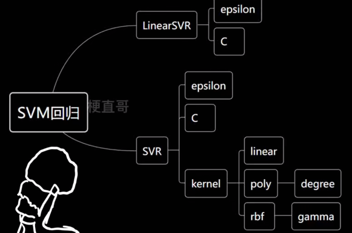
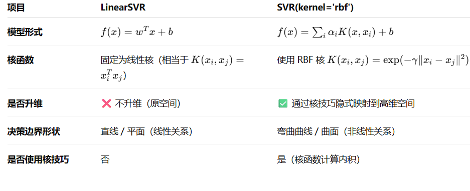
SVM(Support Vector Machine)支持向量机
│
├── 分类任务 → SVC(Support Vector Classification)
│      │
│      ├── LinearSVC(线性分类)
│      └── SVC(kernel='rbf'/'poly'/...)(非线性分类)
│
└── 回归任务 → SVR(Support Vector Regression)│├── LinearSVR(线性回归)└── SVR(kernel='rbf'/'poly'/...)(非线性回归)
SVM核心思想和原理
假设我们有两类点(红色、蓝色):
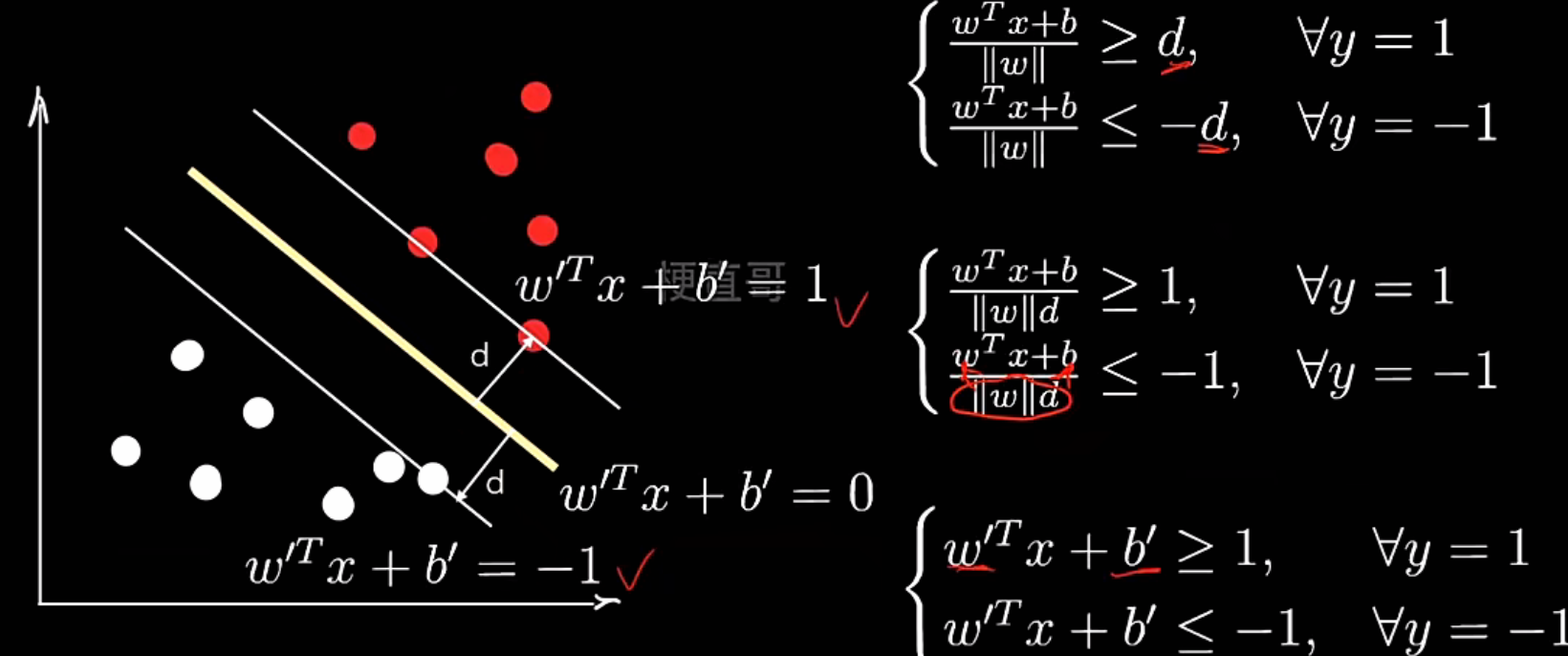
蓝 ● ● ●↑│ ← 这条线(或平面)就是分类边界│红 ● ● ●
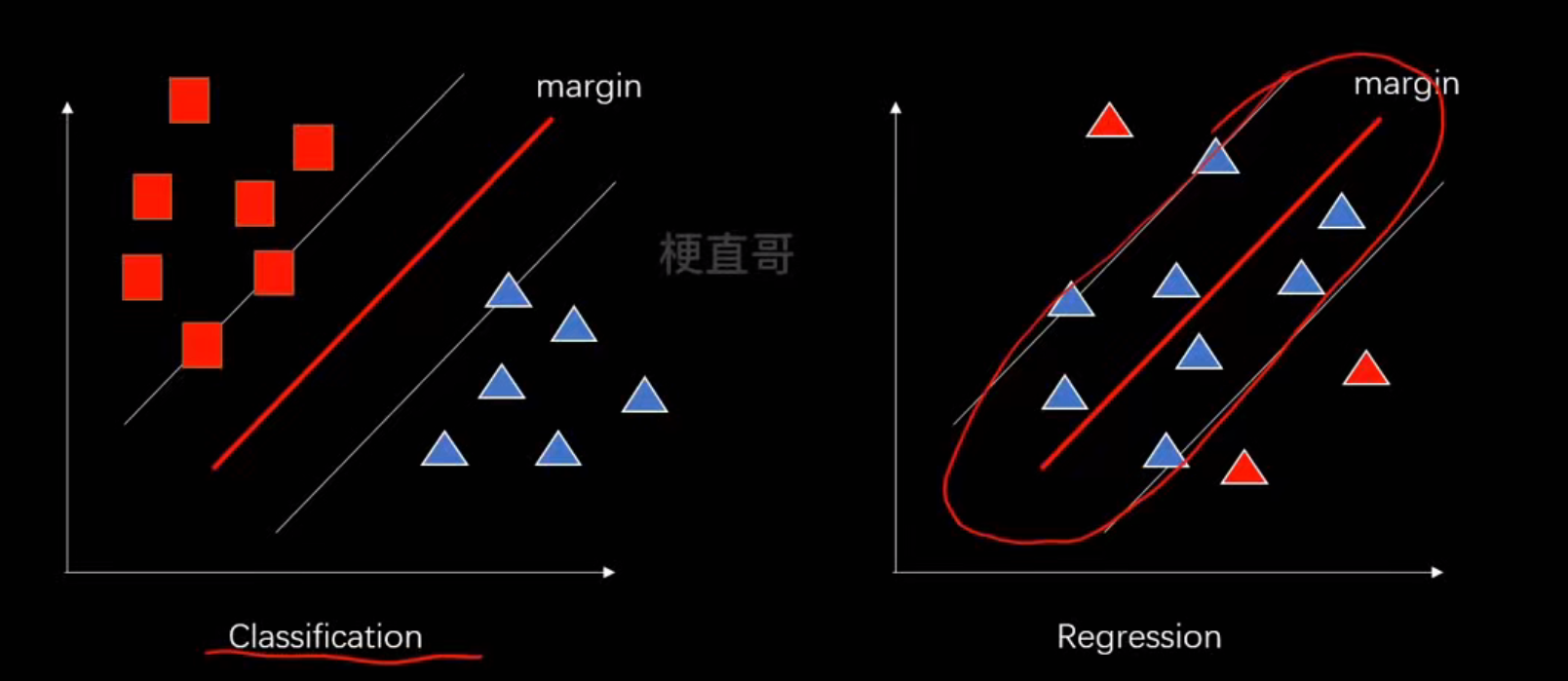
SVM 的目标就是找到一个分割超平面(Hyperplane),把两类样本分开,同时尽可能让两边离这条线最远
核心思想:最大化间隔(margin)-------不仅要能分开数据,还要“分得稳”,也就是要有最大安全距离
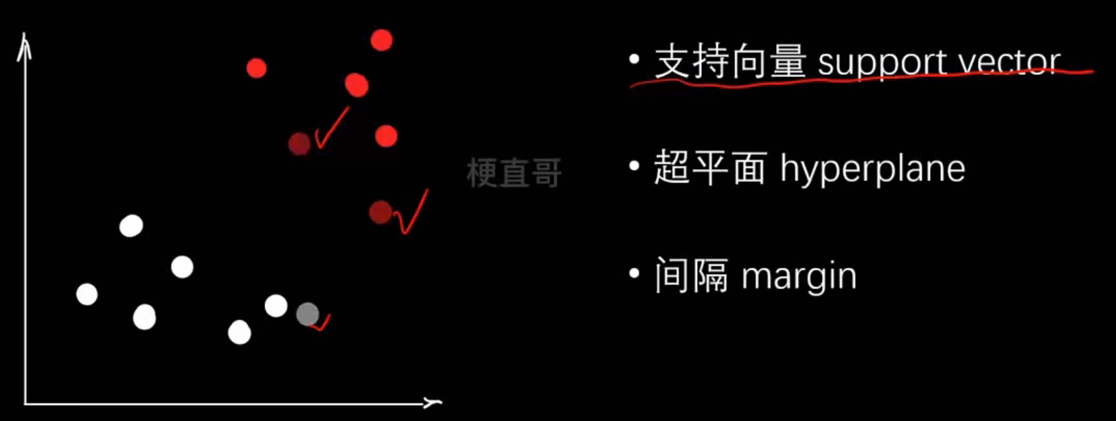
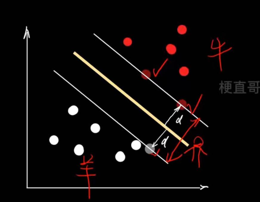
| 步骤 | 图中含义 | 数学含义 |
|---|---|---|
| 1️⃣ 拿到数据 | 红点 vs 白点 | 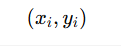 |
| 2️⃣ 假设一条线 | 黄色线 | 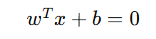 |
| 3️⃣ 计算每个点到线的距离 | 红色箭头 (d) | |
| 4️⃣ 最大化两类点的最小距离 | 白色线之间的距离 | 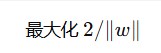 |
| 5️⃣ 得到支持向量 | 靠近白线的点 | 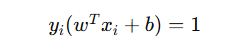 |
支持向量机就是:在所有能分开两类样本的线中,找那条离两类最近样本最远的线
与线性模型对比:
| 模型 | 分类标准 | 核心思想 | 优化化目标 | 泛化能力 |
|---|---|---|---|---|
| 线性模型 | 决策边界 | 民主投票 | 点到直线距离和 | 一般 |
| SVM | 超平面 | 民主集中 | margin | 提升 |
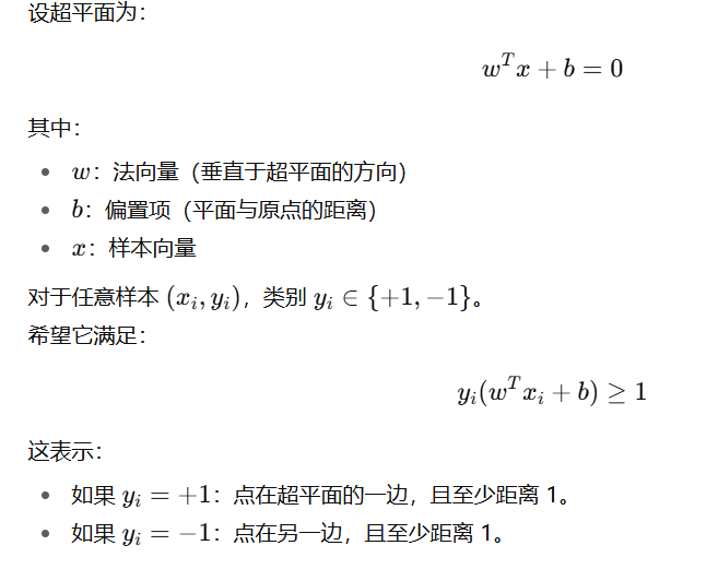
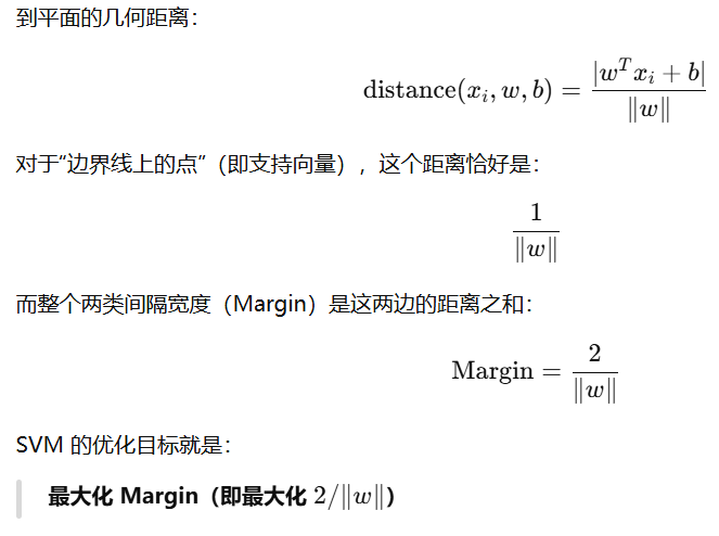
硬间隔SVM
最大间隔超平面:
间隔margin:
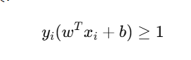
“硬”表示 所有样本都必须严格正确分类。换句话说,任何样本点都不能违反约束:
不允许有:
- 误分类;
- 落在 margin 区域内的点。
因此,它假设数据是完全线性可分的
说白了硬间隔 SVM本质上就是一个带不等式约束的最优化问题
SVM软间隔
- 什么是软间隔?
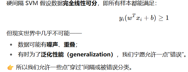
软间隔 SVM 是在“最大化间隔”和“最小化分类错误”之间找到最佳平衡的凸优化问题。
建立容错机制,进一步提升泛化能力
其核心思想是:允许犯错,但要付出代价
- 如何做到?
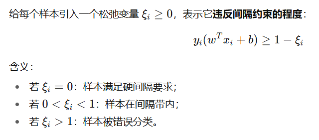
引入松弛变量:
- 目标函数如何权衡”间隔最大化“和”错误最小化“?
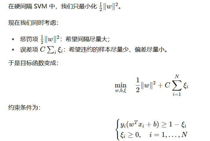
C 控制“间隔宽度”和“错误容忍”的平衡:
- C 大 → 惩罚错误更重 → 模型更严格,倾向于小间隔、低训练误差(可能过拟合)
- C 小 → 允许更多误差 → 间隔更宽,倾向于高泛化能力(可能欠拟合)
可以这么理解:C 就是“惩罚系数”,相当于老师对犯错的学生到底严不严格
线性SVM分类任务代码实现
# 数据集
import numpy as np
import matplotlib.pyplot as plt
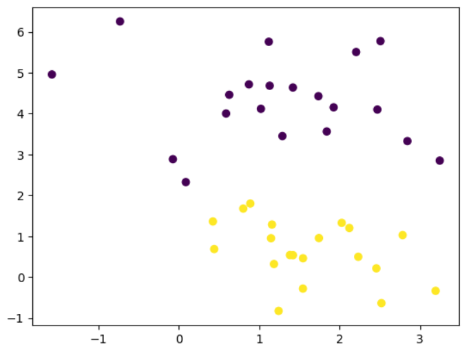
from sklearn.datasets import make_blobsx,y=make_blobs(n_samples=40,centers=2,random_state=0
)plt.scatter(x[:,0],x[:,1],c=y)
plt.show()
# sklearn中的线性SVM
from sklearn.svm import LinearSVC
clf=LinearSVC(C=1)
clf.fit(x,y)
clf.score(x,y)  #1.0
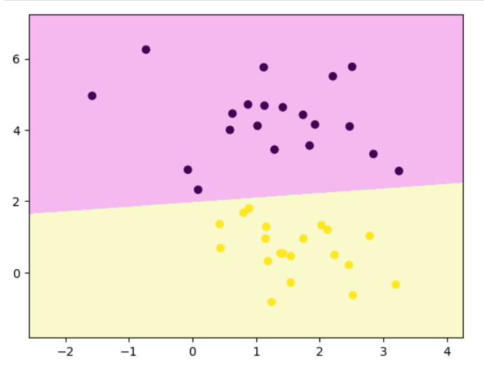
# 画决策边界
def decision_boundary_plot(X, y, clf):axis_x1_min, axis_x1_max = X[:,0].min() - 1, X[:,0].max() + 1axis_x2_min, axis_x2_max = X[:,1].min() - 1, X[:,1].max() + 1x1, x2 = np.meshgrid( np.arange(axis_x1_min,axis_x1_max, 0.01) , np.arange(axis_x2_min,axis_x2_max, 0.01))z = clf.predict(np.c_[x1.ravel(),x2.ravel()])z = z.reshape(x1.shape)from matplotlib.colors import ListedColormapcustom_cmap = ListedColormap(['#F5B9EF','#BBFFBB','#F9F9CB'])plt.contourf(x1, x2, z, cmap=custom_cmap)plt.scatter(X[:,0], X[:,1], c=y)plt.show()
decision_boundary_plot(x,y,clf)
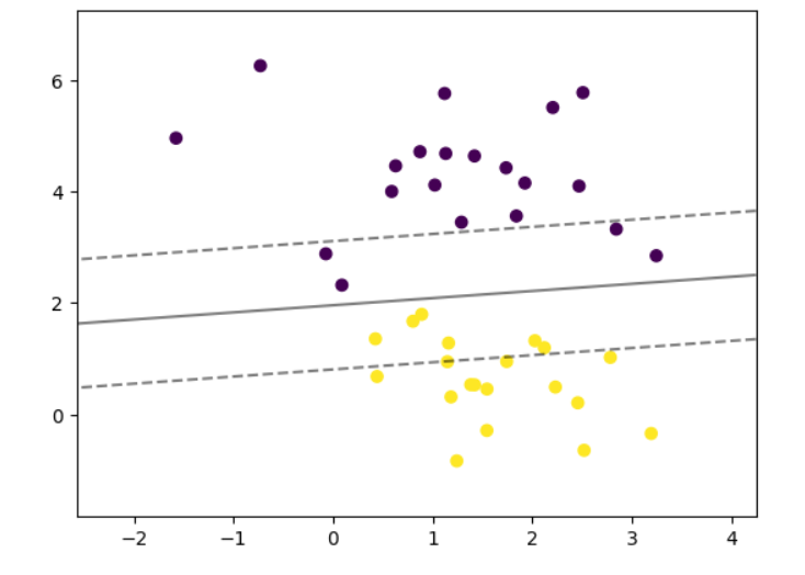
# 可视化支持向量机(SVM)的决策边界和间隔线
def plot_svm_margin(x, y, clf, ax = None):from sklearn.inspection import DecisionBoundaryDisplayDecisionBoundaryDisplay.from_estimator(clf,x,ax = ax,grid_resolution=50,plot_method="contour",colors="k",levels=[-1, 0, 1],alpha=0.5,linestyles=["--", "-", "--"],)plt.scatter(x[:,0], x[:,1], c = y)
plot_svm_margin(x,y,clf)
plt.show()
# 依次看一下不同的C值对分类的影响
plt.rcParams["figure.figsize"] = (12, 8)params = [0.1, 1, 10, 100]
for i, c in enumerate(params):clf = LinearSVC(C = c, random_state=0)clf.fit(x, y)ax = plt.subplot(2, 2, i + 1)plt.title("C: {0}".format(c))plot_svm_margin(x, y, clf, ax)plt.show()
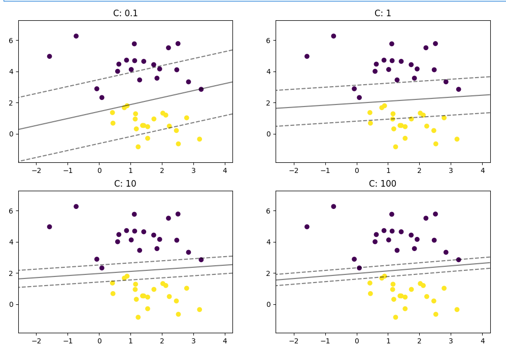
由图分析:
| C 值 | 惩罚强度 | 间隔宽度 | 分类精度 | 泛化表现 |
|---|---|---|---|---|
| 小 (0.1) | 低(容错高) | 宽 | 错误多 | 稳定但欠拟合 |
| 中 (1) | 适中 | 合理 | 平衡 | 泛化最好 |
| 大 (10–100) | 高(严苛) | 窄 | 训练集高精度 | 容易过拟合 |
# 支持向量机解决多分类
from sklearn import datasetsiris=datasets.load_iris()
x=iris.data
y=iris.target
clf=LinearSVC(C=0.1,multi_class='ovr',random_state=0)
clf.fit(x,y)clf.predict(x)
# 看看准确率
from sklearn.metrics import accuracy_score
accuracy = accuracy_score(y, clf.predict(x))
print("准确率:", accuracy)   #0.96
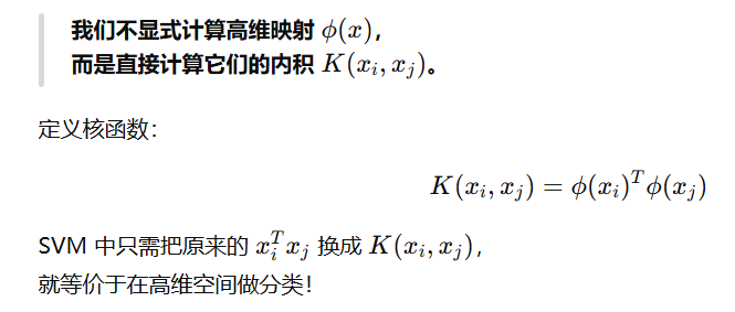
非线性SVM:核技巧
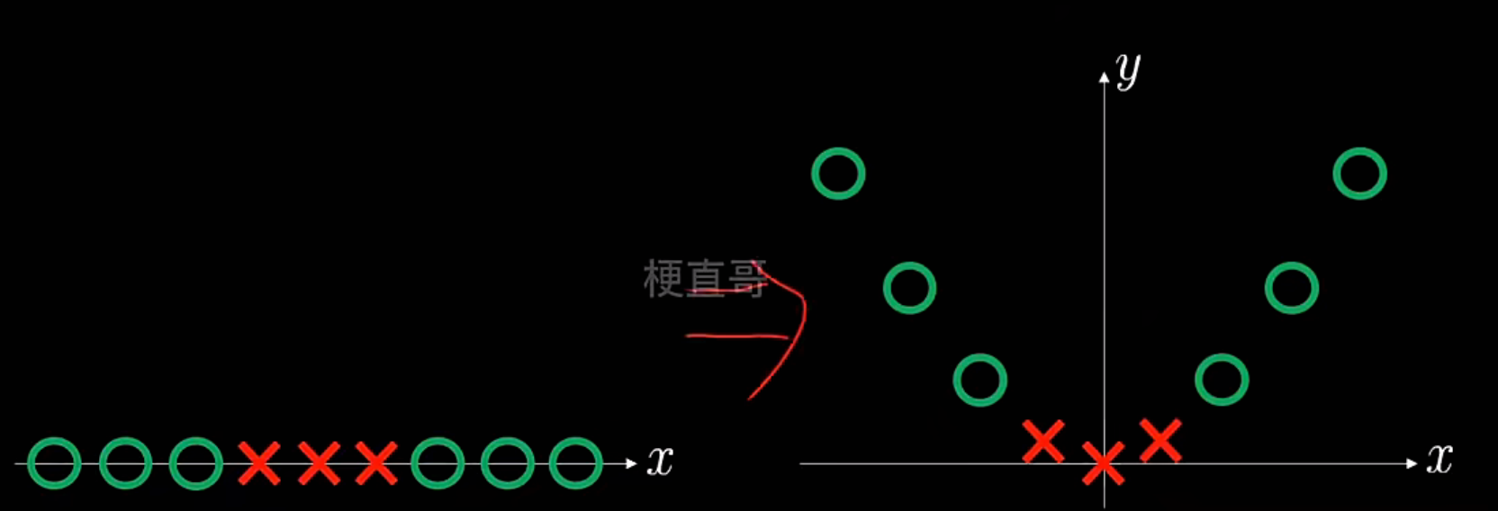
线性不可分问题:
怎么解决?升维映射
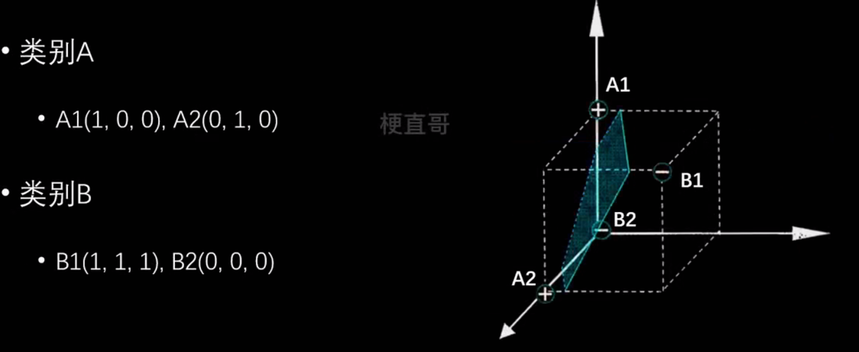
核技巧:

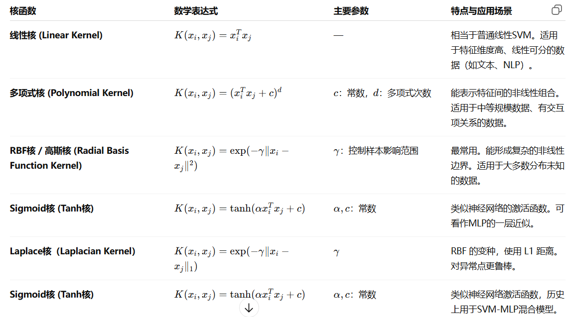
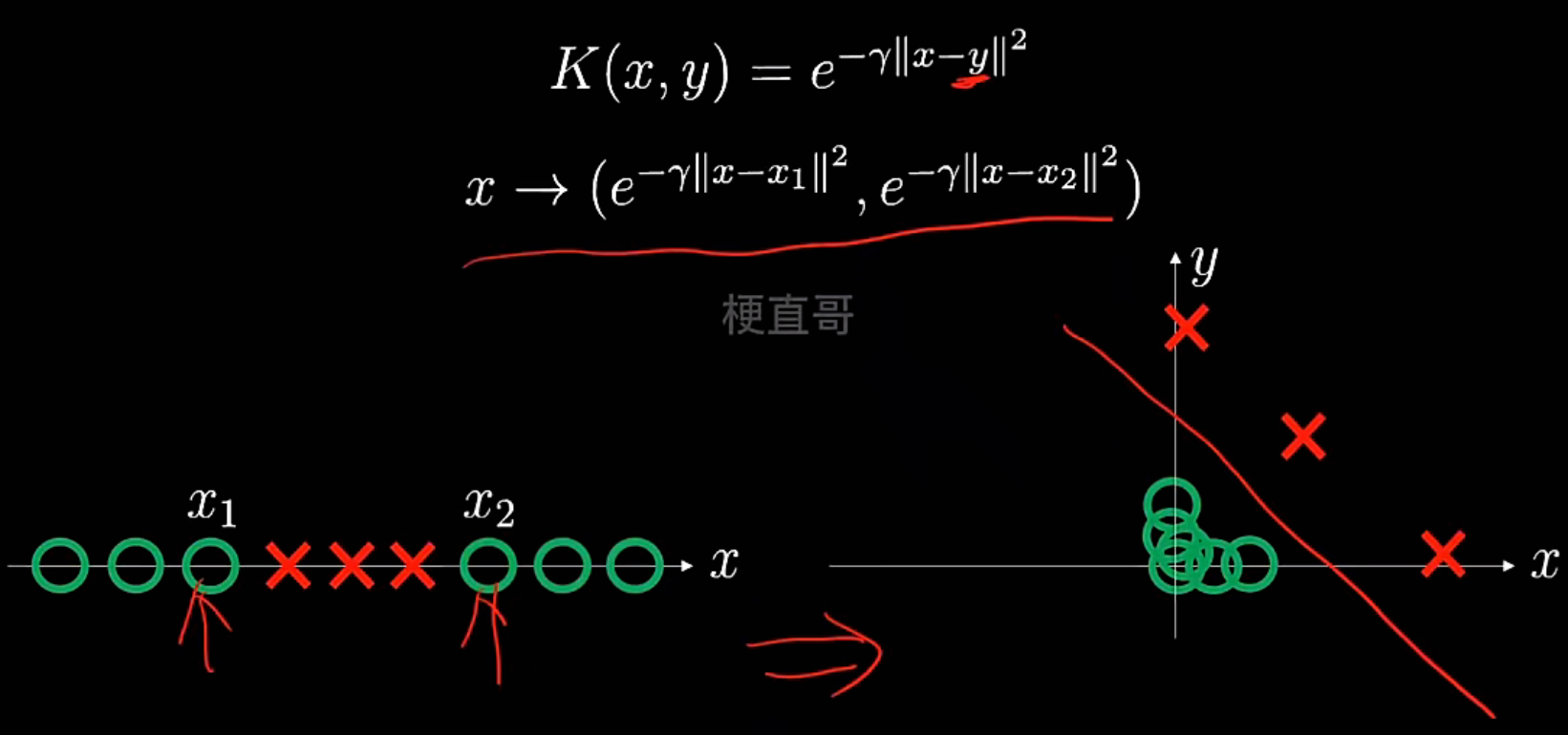
常用核函数:
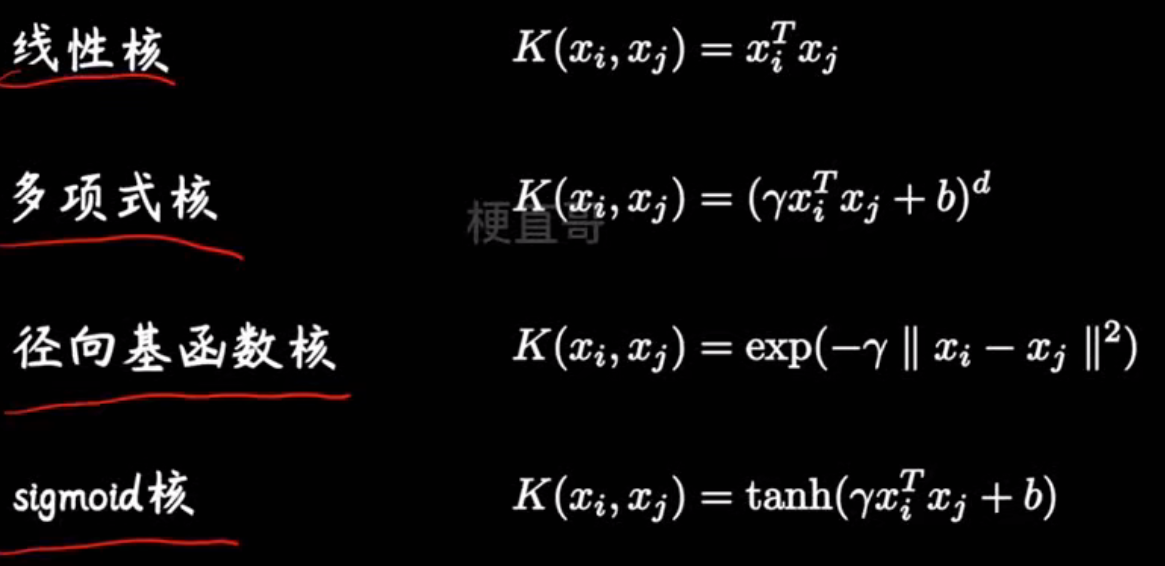
SVM核函数
此处讲讲多项式核函数:
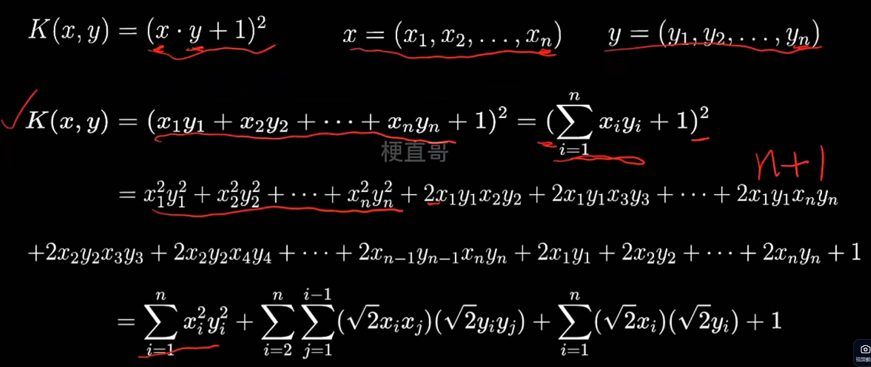
多项式核解决非线性
高斯核函数解决非线性问题
非线性SVM分类任务代码实现
| 对比项 | 线性 SVM | 非线性 SVM |
|---|---|---|
| 数据分布 | 样本在原空间中线性可分 | 样本在原空间中线性不可分 |
| 决策边界 | 一条直线 / 超平面 | 一条曲线 / 曲面(在原空间) |
| 思想 | 直接在原空间找最大间隔超平面 | 先隐式映射到高维空间,再找线性超平面(核函数) |
| 几何效果 | 平面划分两类 | 高维超平面在原空间表现为非线性边界 |
# 数据集----这是线性不可分模型
import numpy as np
import matplotlib.pyplot as pltfrom sklearn.datasets import make_moons
# make_moons生成非线性数据
x, y = make_moons(n_samples=100, noise=0.2, random_state=0)plt.scatter(x[:,0], x[:,1], c = y)
plt.show()
# 线性 SVM 决策边界可视化函数
from sklearn.svm import LinearSVClsvc = LinearSVC()
lsvc.fit(x,y)def decision_boundary_plot(X, y, clf):axis_x1_min, axis_x1_max = X[:,0].min() - 1, X[:,0].max() + 1axis_x2_min, axis_x2_max = X[:,1].min() - 1, X[:,1].max() + 1x1, x2 = np.meshgrid( np.arange(axis_x1_min,axis_x1_max, 0.01) , np.arange(axis_x2_min,axis_x2_max, 0.01))z = clf.predict(np.c_[x1.ravel(),x2.ravel()])z = z.reshape(x1.shape)from matplotlib.colors import ListedColormapcustom_cmap = ListedColormap(['#F5B9EF','#BBFFBB','#F9F9CB'])plt.contourf(x1, x2, z, cmap=custom_cmap)plt.scatter(X[:,0], X[:,1], c=y)plt.show()decision_boundary_plot(x,y,lsvc)
显式多项式升维 + 线性 SVM
from sklearn.preprocessing import PolynomialFeatures, StandardScaler
from sklearn.pipeline import Pipeline
poly_svc = Pipeline([("poly", PolynomialFeatures(degree=3)),  #拐两个弯("std_scaler", StandardScaler()),("linearSVC", LinearSVC())
])poly_svc.fit(x,y)decision_boundary_plot(x,y,poly_svc)
代码里的 LinearSVC 确实是 线性核 SVM,但由于前面加了 PolynomialFeatures(degree=3),整体模型相当于在高维多项式空间中训练线性 SVM,在原始特征空间表现为一个 非线性(弯曲)决策边界。
多项式核函数解决非线性问题
| 参数 | 作用 | 默认值 | 说明 |
|---|---|---|---|
degree | 多项式的次数 (d) | 3 | 决定映射的“弯曲复杂度” |
coef0 | 常数项 ® | 0 | 决定低阶项与高阶项的权重 |
gamma | 核宽度系数 | 'scale' | 控制特征缩放(和 RBF 类似) |
# 多项式核 SVM
from sklearn.svm import SVC
poly_svc = Pipeline([("std_scaler", StandardScaler()),("polySVC", SVC(kernel='poly', degree=3, coef0=5 ))
])
poly_svc.fit(x,y)
decision_boundary_plot(x,y,poly_svc)
高斯核函数
sigma越大,曲线越平缓
rbf_svc = Pipeline([("std_scaler", StandardScaler()),("rbfSVC", SVC(kernel='rbf', gamma=0.1 ))
])rbf_svc.fit(x,y)
decision_boundary_plot(x,y,rbf_svc)
rbf_svc = Pipeline([("std_scaler", StandardScaler()),("rbfSVC", SVC(kernel='rbf', gamma=10 ))
])
rbf_svc.fit(x,y)
decision_boundary_plot(x,y,rbf_svc)
rbf_svc = Pipeline([("std_scaler", StandardScaler()),("rbfSVC", SVC(kernel='rbf', gamma=100 ))
])
rbf_svc.fit(x,y)
decision_boundary_plot(x,y,rbf_svc)
| γ 的取值(gamma) | 样本的“影响半径” | 决策边界 | 模型复杂度 | 泛化能力 |
|---|---|---|---|---|
| 小(如 0.1) | 每个样本影响范围大 | 边界平滑 | 简单 | 泛化强(但可能欠拟合) |
| 中(如 10) | 影响范围适中 | 边界适度弯曲 | 较复杂 | 泛化良好 |
| 大(如 100) | 每个样本只影响极近邻 | 边界剧烈弯曲 | 极复杂 | 容易过拟合 |
如何选择核函数?
- 当特征多且接近样本数量,可直接选择线性核SVM
- 当特征数少,样本数正常,推荐选择高斯核函数
- 当特征数少,样本数很大,建议选择多项式核函数
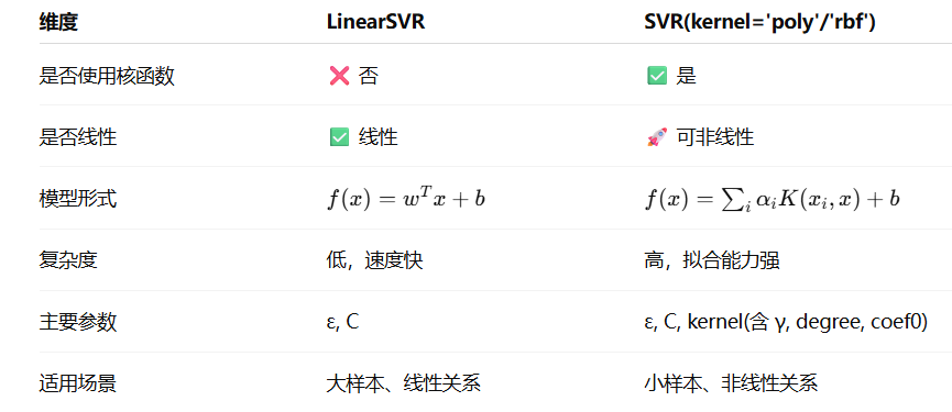
SVM回归任务代码实现
SVM回归分两类:
| 类型 | 说明 |
|---|---|
| LinearSVR | 线性支持向量回归(不使用核函数) |
| SVR | 核支持向量回归(可使用多种核函数,如 RBF、多项式等) |
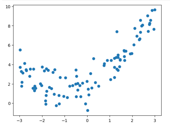
# 数据集
import numpy as np
import matplotlib.pyplot as pltnp.random.seed(666)
x = np.random.uniform(-3,3,size=100)
y = 0.5 * x**2 +x +2 +np.random.normal(0,1,size=100)
X = x.reshape(-1,1)plt.scatter(x,y)
plt.show()
# 线性SVR
# 线性支持向量回归
from sklearn.svm import LinearSVR
from sklearn.preprocessing import StandardScaler
from sklearn.pipeline import Pipelinedef StandardLinearSVR(epsilon=0.1):return Pipeline([("std_scaler",StandardScaler()),("linearSVR",LinearSVR(epsilon=epsilon))])svr = StandardLinearSVR()
svr.fit(X,y)
y_predict = svr.predict(X)
plt.scatter(x,y)
plt.plot(np.sort(x),y_predict[np.argsort(x)],color='r')
plt.show()svr.score(X,y)  #0.48764762540009954
# RBF核SVR
# 带 RBF 核的支持向量回归
from sklearn.svm import SVR
def StandardSVR(epsilon=0.1):return Pipeline([('std_scaler',StandardScaler()),('SVR',SVR(kernel='rbf',epsilon=epsilon))   #高斯核函数])
svr = StandardSVR()
svr.fit(X,y)
y_predict = svr.predict(X)
plt.scatter(x,y)
plt.plot(np.sort(x),y_predict[np.argsort(x)],color='r')
plt.show()svr.score(X,y)  # 0.8138647789256848
SVM优缺点和适用条件
优点:
- 高效处理非线性数据
- 良好的泛化能力
- 解决分类和回归问题
- 稳定性
缺点:
- 选择合适的核函数比较困难
- 大量内存需求
- 大数据集上训练时间长
- 难以解释
7、集成学习
团结就是力量
日常生活中普遍存在的决策思想
兼听则明,偏信则暗
集成学习核心思想和原理
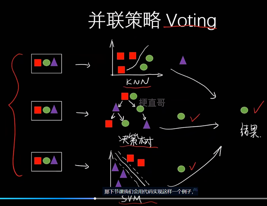
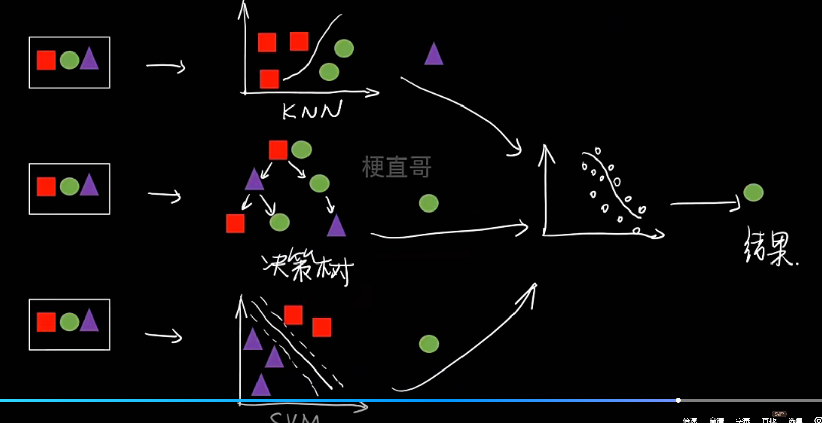
与其依赖一个复杂的模型,不如集合多个相对简单(或不同)的模型,通过某种方式将它们的结果组合起来,从而获得一个更强大、更稳定、更精确的最终模型
既可以监督学习,也可以无监督学习
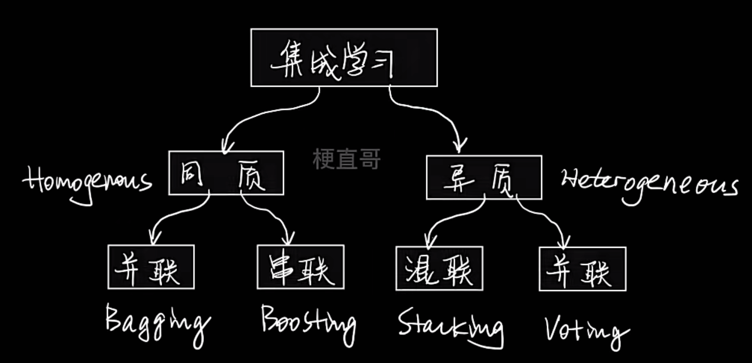
- 同质
- 含义:所有基学习器都是同一种类型的模型,比如全是决策树,或者全是神经网络
- 举例:随机森林(全是决策树)、AdaBoost(通常使用决策树桩)
- 异质
- 含义:基学习器是不同类型的模型,比如一个支持向量机 + 一个决策树 + 一个逻辑回归模型。
- 举例:Voting 和 Stacking 方法常使用异质学习器
- 并联
- 含义:所有基学习器可以独立、并行地进行训练。它们之间没有依赖关系。
- 代表算法:Bagging 和 Voting(少数服从多数)
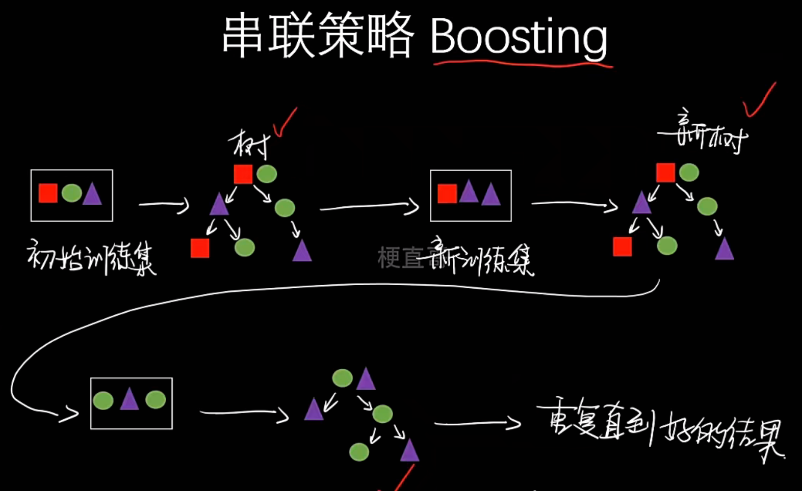
- 串联
- 含义:基学习器需要按顺序依次训练。后一个学习器的训练依赖于前一个学习器的结果(比如,重点关注前一个学习器分错的样本)
- 代表算法:Boosting
- 混联
- 含义:结合了并联和串联的特点,是一种更复杂的层次化结构
- 代表算法:Stacking。它第一层是多个并联的基学习器(可以是同质或异质),第二层再串联一个元学习器来整合第一层的结果
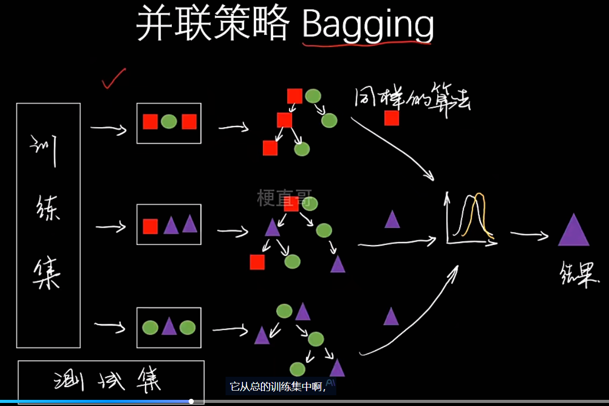
- Bagging
- 类型:同质
- 组合方式:并联
- 核心思想:通过自助采样训练多个模型,然后“投票”或“平均”结果。旨在降低方差,防止过拟合
- 典型代表:随机森林
- Boosting
- 类型:同质
- 组合方式:串联
- 核心思想:顺序训练模型,后续模型专注于修正前序模型的错误。旨在降低偏差,提升模型精度
- 典型代表:AdaBoost, GBDT, XGBoost, LightGBM
- Stacking
- 类型:通常为异质(也可以是同质)
- 组合方式:混联(先并联,后串联)
- 核心思想:训练多个不同的基模型,然后将它们的预测结果作为新的特征,再训练一个“元模型”来进行最终决策。旨在博采众长。
集成学习代码实现
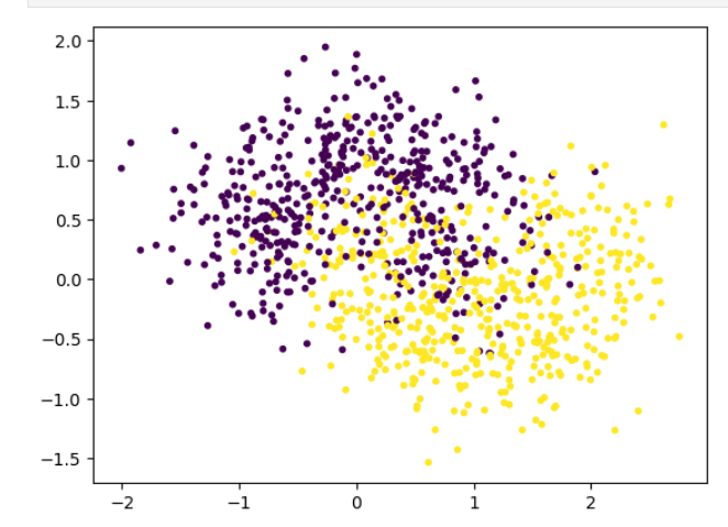
# 数据集
import numpy as np
import matplotlib.pyplot as plt
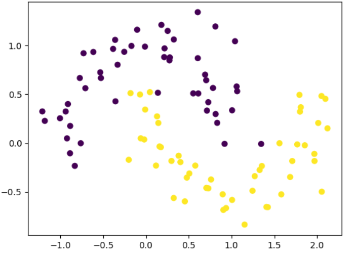
from sklearn.datasets import make_moonsx,y=make_moons(n_samples=1000,noise=0.4,random_state=20
)
x.shape,y.shape输出:
((1000, 2), (1000,))plt.scatter(x[:,0],x[:,1],c=y,s=10)
plt.show()
from sklearn.model_selection import train_test_split
x_train,x_test,y_train,y_test=train_test_split(x,y,random_state=0)
# 手动实现集成学习的分类器
# 创建三个不同的分类器from sklearn.neighbors import KNeighborsClassifier
from sklearn.linear_model import LogisticRegression
from sklearn.naive_bayes import GaussianNBclf=[KNeighborsClassifier(n_neighbors=3),LogisticRegression(),GaussianNB()
]
# 打印分类器在测试集上的score
for i in range(len(clf)):clf[i].fit(x_train,y_train)print(clf[i].score(x_test,y_test))输出:
0.832
0.848
0.848
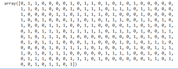
# 三个分类器分别预测到的投票的结果
y_pred=np.zeros_like(y_test)
# 三个分类器分别对测试集进行预测
# 每个分类器的预测结果(0或1)被累加到 y_pred 中
# 最终 y_pred 中每个位置的值表示"有多少个分类器预测该样本为类别1"
for i in range(len(clf)):y_pred+=clf[i].predict(x_test)
y_pred[y_pred<2]=0
y_pred[y_pred>=2]=1
y_pred
from sklearn.metrics import accuracy_score
accuracy_score(y_test,y_pred)输出:
0.852
# 使用sklearn中的集成学习方法
from sklearn.ensemble import VotingClassifier
clf=[KNeighborsClassifier(n_neighbors=3),LogisticRegression(),GaussianNB()
]vclf=VotingClassifier(estimators=[('knn',clf[0]),('lr',clf[1]),('gnb',clf[2])],# 每个基分类器独立预测,最终结果采用"少数服从多数"原则voting='hard',# 并行处理参数n_jobs=-1
)
vclf.fit(x_train,y_train)
vclf.score(x_test,y_test)输出:
0.852
但这种投票策略存在问题:
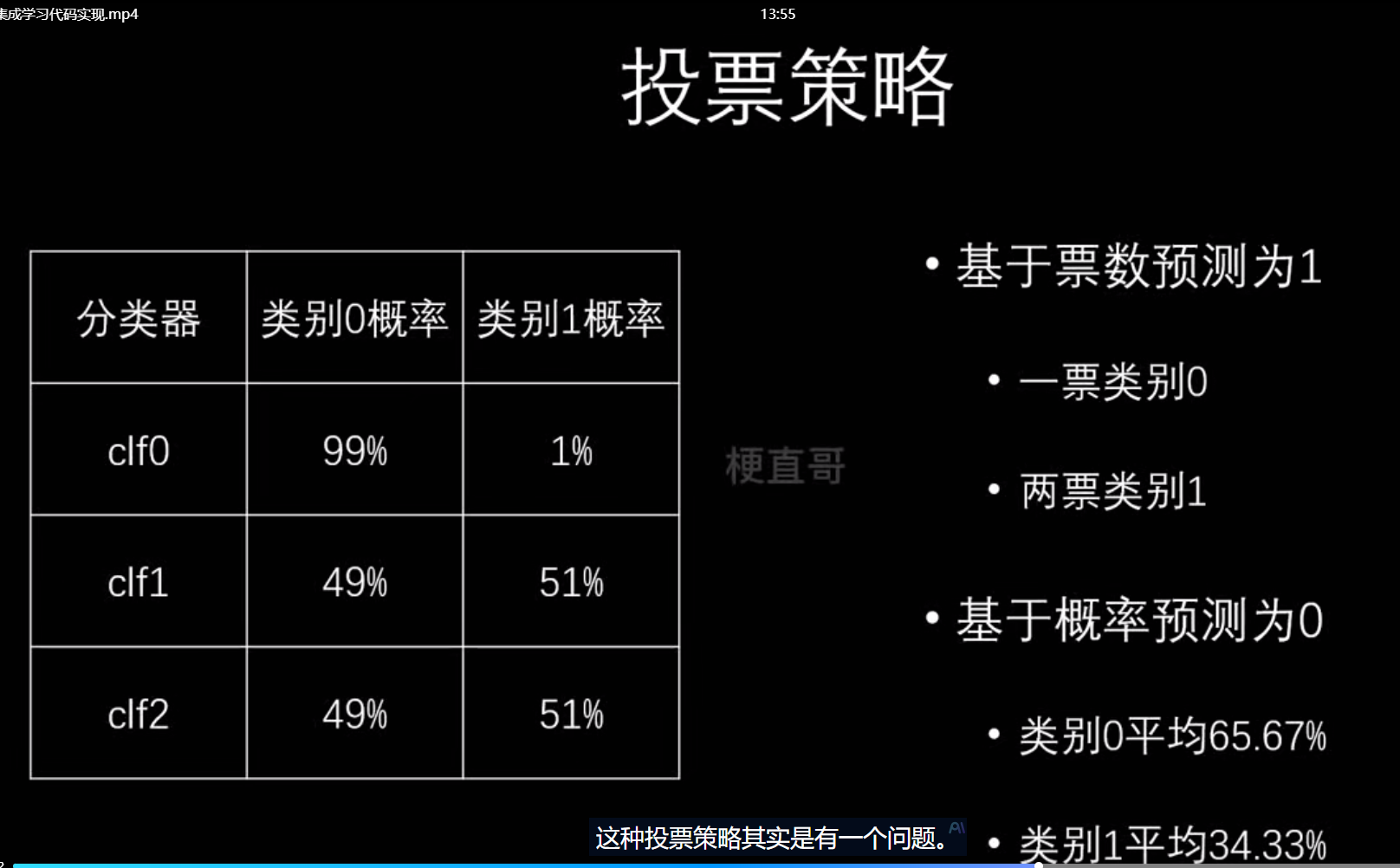
于是我们采用另一种情况:概率求和或者看平均值作为置信度
soft表示软投票,即
# 每个分类器给出属于每个类别的概率
KNN: [P(0)=0.3, P(1)=0.7]    # 预测为1的概率是0.7
LR:  [P(0)=0.6, P(1)=0.4]    # 预测为1的概率是0.4
NB:  [P(0)=0.2, P(1)=0.8]    # 预测为1的概率是0.8# 平均概率
平均P(0) = (0.3 + 0.6 + 0.2) / 3 = 0.37
平均P(1) = (0.7 + 0.4 + 0.8) / 3 = 0.63# 最终选择概率更高的类别
最终结果: 1 (因为0.63 > 0.37)
# 获取概率:每个分类器输出属于各个类别的概率
# 平均概率:计算所有分类器概率的平均值
# 选择类别:选择平均概率最高的类别作为最终预测
vclf=VotingClassifier(estimators=[('knn',clf[0]),('lr',clf[1]),('gnb',clf[2])],voting='soft',# 并行处理参数n_jobs=-1
)
vclf.fit(x_train,y_train)
vclf.score(x_test,y_test)输出:
0.868