EfficientNet模型：高效卷积神经网络的革命性突破

EfficientNet模型：高效卷积神经网络的革命性突破

🌟 你好，我是 励志成为糕手 ！
🌌 在代码的宇宙中，我是那个追逐优雅与性能的星际旅人。
✨ 每一行代码都是我种下的星光，在逻辑的土壤里生长成璀璨的银河；
🛠️ 每一个算法都是我绘制的星图，指引着数据流动的最短路径；
🔍 每一次调试都是星际对话，用耐心和智慧解开宇宙的谜题。
🚀 准备好开始我们的星际编码之旅了吗？

摘要

作为一名深度学习的探索者，我在研究卷积神经网络的道路上遇到了一个令人兴奋的里程碑——EfficientNet。这个模型彻底改变了我对网络设计的认知，它不仅在ImageNet上刷新了准确率记录，更重要的是用更少的参数和计算量达到了前所未有的效果。

EfficientNet的核心思想让我深深着迷：通过复合缩放（Compound Scaling）方法，同时优化网络的深度、宽度和分辨率，而不是传统的单一维度扩展。这种设计哲学就像是在三维空间中寻找最优解，而不是在单一轴线上盲目前进。当我第一次看到EfficientNet-B7在ImageNet上达到84.4%的top-1准确率，同时参数量比GPipe少8.4倍时，我意识到这不仅仅是一个模型的改进，而是整个网络设计范式的革新。

在实际项目中，我发现EfficientNet的魅力远不止于此。它的MBConv（Mobile Inverted Bottleneck Convolution）模块巧妙地结合了深度可分离卷积和Squeeze-and-Excitation注意力机制，让每一层都能高效地提取特征。更令人惊喜的是，通过神经架构搜索（NAS）技术找到的基础架构EfficientNet-B0，为后续的缩放提供了坚实的基础。这种从B0到B7的系统性扩展，让我们可以根据不同的计算资源和精度需求，选择最适合的模型变体。

1. EfficientNet核心原理

1.1 复合缩放方法

EfficientNet最大的创新在于提出了复合缩放方法。传统的网络扩展通常只关注单一维度，要么增加深度，要么增加宽度，要么提高输入分辨率。但EfficientNet认为这三个维度应该协调发展。

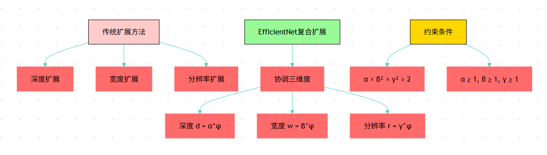
图1：EfficientNet复合缩放方法对比流程图

1.2 缩放系数的数学原理

复合缩放的核心公式非常优雅：

# EfficientNet复合缩放核心实现
import mathclass CompoundScaling:def __init__(self, alpha=1.2, beta=1.1, gamma=1.15):"""初始化复合缩放参数alpha: 深度缩放系数beta: 宽度缩放系数  gamma: 分辨率缩放系数"""self.alpha = alphaself.beta = betaself.gamma = gamma# 验证约束条件：α × β² × γ² ≈ 2constraint = alpha * (beta ** 2) * (gamma ** 2)print(f"约束条件验证: {constraint:.3f} ≈ 2.0")def scale_network(self, phi, base_depth=7, base_width=1.0, base_resolution=224):"""根据复合系数φ缩放网络"""# 计算缩放后的维度scaled_depth = math.ceil(self.alpha ** phi * base_depth)scaled_width = self.beta ** phi * base_widthscaled_resolution = int(self.gamma ** phi * base_resolution)return {'depth': scaled_depth,'width': scaled_width,'resolution': scaled_resolution,'phi': phi}# 演示不同EfficientNet变体的缩放
scaler = CompoundScaling()# 生成B0到B7的配置
efficientnet_configs = {}
for i in range(8):config = scaler.scale_network(phi=i)efficientnet_configs[f'B{i}'] = configprint(f"EfficientNet-B{i}: 深度={config['depth']}, "f"宽度={config['width']:.2f}, 分辨率={config['resolution']}")

2. MBConv模块架构

2.1 移动倒置瓶颈卷积

MBConv是EfficientNet的基础构建块，它巧妙地结合了多种先进技术：

图2：MBConv模块处理时序图

2.2 MBConv模块实现

import torch
import torch.nn as nn
import torch.nn.functional as Fclass SEBlock(nn.Module):"""Squeeze-and-Excitation注意力模块"""def __init__(self, in_channels, reduction=4):super(SEBlock, self).__init__()self.avg_pool = nn.AdaptiveAvgPool2d(1)self.fc = nn.Sequential(nn.Linear(in_channels, in_channels // reduction, bias=False),nn.ReLU(inplace=True),nn.Linear(in_channels // reduction, in_channels, bias=False),nn.Sigmoid())def forward(self, x):b, c, _, _ = x.size()# 全局平均池化y = self.avg_pool(x).view(b, c)# 通道注意力权重y = self.fc(y).view(b, c, 1, 1)return x * y.expand_as(x)class MBConvBlock(nn.Module):"""Mobile Inverted Bottleneck Convolution Block"""def __init__(self, in_channels, out_channels, kernel_size=3, stride=1, expand_ratio=6, se_ratio=0.25):super(MBConvBlock, self).__init__()self.stride = strideself.use_residual = (stride == 1 and in_channels == out_channels)# 扩展阶段expanded_channels = in_channels * expand_ratioself.expand_conv = nn.Sequential(nn.Conv2d(in_channels, expanded_channels, 1, bias=False),nn.BatchNorm2d(expanded_channels),nn.ReLU6(inplace=True)) if expand_ratio != 1 else nn.Identity()# 深度卷积阶段self.depthwise_conv = nn.Sequential(nn.Conv2d(expanded_channels, expanded_channels, kernel_size, stride, kernel_size//2, groups=expanded_channels, bias=False),nn.BatchNorm2d(expanded_channels),nn.ReLU6(inplace=True))# SE注意力模块self.se_block = SEBlock(expanded_channels, reduction=max(1, int(in_channels * se_ratio)))# 投影阶段self.project_conv = nn.Sequential(nn.Conv2d(expanded_channels, out_channels, 1, bias=False),nn.BatchNorm2d(out_channels))def forward(self, x):identity = x# 扩展x = self.expand_conv(x)# 深度卷积x = self.depthwise_conv(x)# SE注意力x = self.se_block(x)# 投影x = self.project_conv(x)# 残差连接if self.use_residual:x = x + identityreturn x# 测试MBConv模块
def test_mbconv():# 创建测试输入x = torch.randn(2, 32, 56, 56)# 创建MBConv块mbconv = MBConvBlock(in_channels=32, out_channels=64, kernel_size=3, stride=2, expand_ratio=6)# 前向传播output = mbconv(x)print(f"输入形状: {x.shape}")print(f"输出形状: {output.shape}")# 计算参数量total_params = sum(p.numel() for p in mbconv.parameters())print(f"MBConv参数量: {total_params:,}")test_mbconv()

3. EfficientNet完整架构

3.1 网络架构设计

EfficientNet的整体架构遵循了一个精心设计的模式：

图3：EfficientNet整体架构图

3.2 完整网络实现

class EfficientNet(nn.Module):"""EfficientNet主网络"""def __init__(self, num_classes=1000, width_mult=1.0, depth_mult=1.0):super(EfficientNet, self).__init__()# EfficientNet-B0基础配置# [expand_ratio, channels, repeats, stride, kernel_size]self.cfg = [[1,  16,  1, 1, 3],  # Stage 1[6,  24,  2, 2, 3],  # Stage 2[6,  40,  2, 2, 5],  # Stage 3[6,  80,  3, 2, 3],  # Stage 4[6, 112,  3, 1, 5],  # Stage 5[6, 192,  4, 2, 5],  # Stage 6[6, 320,  1, 1, 3],  # Stage 7]# Stem层self.stem = nn.Sequential(nn.Conv2d(3, 32, 3, stride=2, padding=1, bias=False),nn.BatchNorm2d(32),nn.ReLU6(inplace=True))# 构建MBConv层self.blocks = nn.ModuleList()in_channels = 32for expand_ratio, channels, repeats, stride, kernel_size in self.cfg:out_channels = int(channels * width_mult)num_repeats = int(repeats * depth_mult)for i in range(num_repeats):self.blocks.append(MBConvBlock(in_channels=in_channels,out_channels=out_channels,kernel_size=kernel_size,stride=stride if i == 0 else 1,expand_ratio=expand_ratio))in_channels = out_channels# 分类头self.head = nn.Sequential(nn.Conv2d(in_channels, 1280, 1, bias=False),nn.BatchNorm2d(1280),nn.ReLU6(inplace=True),nn.AdaptiveAvgPool2d(1),nn.Flatten(),nn.Dropout(0.2),nn.Linear(1280, num_classes))def forward(self, x):# Stemx = self.stem(x)# MBConv blocksfor block in self.blocks:x = block(x)# Classification headx = self.head(x)return xdef create_efficientnet_b0():"""创建EfficientNet-B0模型"""return EfficientNet(width_mult=1.0, depth_mult=1.0)def create_efficientnet_b1():"""创建EfficientNet-B1模型"""return EfficientNet(width_mult=1.0, depth_mult=1.1)# 模型测试
model = create_efficientnet_b0()
x = torch.randn(1, 3, 224, 224)
output = model(x)
print(f"模型输出形状: {output.shape}")# 计算模型参数量和FLOPs
def count_parameters(model):return sum(p.numel() for p in model.parameters() if p.requires_grad)print(f"EfficientNet-B0参数量: {count_parameters(model):,}")

4. 性能对比分析

4.1 不同模型性能对比

让我们通过表格来对比EfficientNet与其他经典模型的性能：

模型	Top-1准确率(%)	参数量(M)	FLOPs(B)	推理时间(ms)
ResNet-50	76.0	25.6	4.1	32
ResNet-152	78.3	60.2	11.6	87
DenseNet-169	76.2	14.1	3.4	45
MobileNetV2	72.0	3.4	0.3	12
EfficientNet-B0	77.3	5.3	0.4	15
EfficientNet-B1	79.1	7.8	0.7	18
EfficientNet-B7	84.4	66.3	37.0	125

4.2 效率分析图表

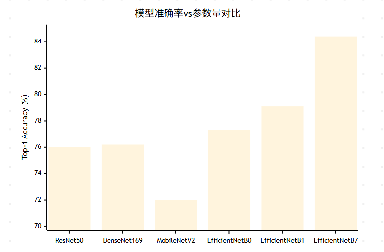
图4：不同模型准确率对比XY图表

5. 训练策略与优化

5.1 渐进式训练策略

EfficientNet的训练采用了渐进式策略，从小分辨率开始逐步增加：

class ProgressiveTraining:"""EfficientNet渐进式训练策略"""def __init__(self, model, initial_size=128, target_size=224):self.model = modelself.initial_size = initial_sizeself.target_size = target_sizeself.current_epoch = 0def get_current_resolution(self, epoch, total_epochs):"""根据训练进度计算当前分辨率"""progress = epoch / total_epochscurrent_size = int(self.initial_size + (self.target_size - self.initial_size) * progress)return current_sizedef create_data_loader(self, dataset, batch_size, resolution):"""创建指定分辨率的数据加载器"""transform = transforms.Compose([transforms.Resize((resolution, resolution)),transforms.RandomHorizontalFlip(),transforms.ToTensor(),transforms.Normalize(mean=[0.485, 0.456, 0.406],std=[0.229, 0.224, 0.225])])dataset.transform = transformreturn DataLoader(dataset, batch_size=batch_size, shuffle=True)# 训练配置
class EfficientNetTrainer:def __init__(self, model, device='cuda'):self.model = model.to(device)self.device = deviceself.optimizer = torch.optim.AdamW(model.parameters(), lr=0.016,  # 基础学习率weight_decay=1e-5)self.scheduler = torch.optim.lr_scheduler.CosineAnnealingLR(self.optimizer, T_max=350)self.criterion = nn.CrossEntropyLoss(label_smoothing=0.1)def train_epoch(self, dataloader, epoch):"""训练一个epoch"""self.model.train()total_loss = 0correct = 0total = 0for batch_idx, (data, target) in enumerate(dataloader):data, target = data.to(self.device), target.to(self.device)# 前向传播self.optimizer.zero_grad()output = self.model(data)loss = self.criterion(output, target)# 反向传播loss.backward()self.optimizer.step()# 统计total_loss += loss.item()pred = output.argmax(dim=1, keepdim=True)correct += pred.eq(target.view_as(pred)).sum().item()total += target.size(0)if batch_idx % 100 == 0:print(f'Epoch: {epoch}, Batch: {batch_idx}, 'f'Loss: {loss.item():.4f}, 'f'Acc: {100.*correct/total:.2f}%')self.scheduler.step()return total_loss / len(dataloader), 100. * correct / total

5.2 数据增强策略

import torchvision.transforms as transforms
from PIL import Image
import randomclass EfficientNetAugmentation:"""EfficientNet专用数据增强"""def __init__(self, image_size=224):self.image_size = image_sizedef get_train_transform(self):"""训练时的数据增强"""return transforms.Compose([transforms.RandomResizedCrop(self.image_size, scale=(0.08, 1.0)),transforms.RandomHorizontalFlip(p=0.5),transforms.ColorJitter(brightness=0.4, contrast=0.4, saturation=0.4, hue=0.1),transforms.ToTensor(),transforms.Normalize(mean=[0.485, 0.456, 0.406],std=[0.229, 0.224, 0.225]),transforms.RandomErasing(p=0.25)  # 随机擦除])def get_val_transform(self):"""验证时的数据变换"""return transforms.Compose([transforms.Resize(int(self.image_size * 1.14)),  # 稍大一些transforms.CenterCrop(self.image_size),transforms.ToTensor(),transforms.Normalize(mean=[0.485, 0.456, 0.406],std=[0.229, 0.224, 0.225])])# AutoAugment策略
class AutoAugment:"""AutoAugment数据增强策略"""def __init__(self):self.policies = [# 策略1: 旋转 + 等化[('rotate', 0.9, 9), ('equalize', 0.8, 6)],# 策略2: 色彩 + 等化  [('color', 0.4, 0), ('equalize', 0.6, 7)],# 更多策略...]def __call__(self, img):policy = random.choice(self.policies)for operation, probability, magnitude in policy:if random.random() < probability:img = self.apply_operation(img, operation, magnitude)return imgdef apply_operation(self, img, operation, magnitude):"""应用具体的增强操作"""if operation == 'rotate':angle = magnitude * 30 / 10  # 映射到角度return img.rotate(angle)elif operation == 'equalize':return transforms.functional.equalize(img)# 其他操作...return img

6. 实际应用案例

6.1 图像分类任务

class ImageClassifier:"""基于EfficientNet的图像分类器"""def __init__(self, model_name='efficientnet-b0', num_classes=1000):self.model = self.load_pretrained_model(model_name, num_classes)self.transform = self.get_transform()def load_pretrained_model(self, model_name, num_classes):"""加载预训练模型"""# 这里可以使用timm库或自定义实现model = create_efficientnet_b0()# 如果类别数不是1000，需要修改分类头if num_classes != 1000:model.head[-1] = nn.Linear(1280, num_classes)return modeldef get_transform(self):"""获取预处理变换"""return transforms.Compose([transforms.Resize(256),transforms.CenterCrop(224),transforms.ToTensor(),transforms.Normalize(mean=[0.485, 0.456, 0.406],std=[0.229, 0.224, 0.225])])def predict(self, image_path):"""预测单张图片"""# 加载图片image = Image.open(image_path).convert('RGB')# 预处理input_tensor = self.transform(image).unsqueeze(0)# 推理self.model.eval()with torch.no_grad():outputs = self.model(input_tensor)probabilities = F.softmax(outputs, dim=1)predicted_class = torch.argmax(probabilities, dim=1).item()confidence = probabilities[0][predicted_class].item()return predicted_class, confidencedef batch_predict(self, image_paths, batch_size=32):"""批量预测"""results = []for i in range(0, len(image_paths), batch_size):batch_paths = image_paths[i:i+batch_size]batch_tensors = []for path in batch_paths:image = Image.open(path).convert('RGB')tensor = self.transform(image)batch_tensors.append(tensor)# 批量推理batch_input = torch.stack(batch_tensors)self.model.eval()with torch.no_grad():outputs = self.model(batch_input)probabilities = F.softmax(outputs, dim=1)for j, prob in enumerate(probabilities):predicted_class = torch.argmax(prob).item()confidence = prob[predicted_class].item()results.append((batch_paths[j], predicted_class, confidence))return results# 使用示例
classifier = ImageClassifier(num_classes=10)  # 假设10类分类任务
# predicted_class, confidence = classifier.predict('test_image.jpg')
# print(f"预测类别: {predicted_class}, 置信度: {confidence:.4f}")

6.2 迁移学习应用

图5：EfficientNet迁移学习用户旅程图

7. 模型优化与部署

7.1 模型量化

import torch.quantization as quantizationclass EfficientNetQuantization:"""EfficientNet模型量化"""def __init__(self, model):self.model = modeldef post_training_quantization(self, calibration_loader):"""训练后量化"""# 设置量化配置self.model.eval()self.model.qconfig = quantization.get_default_qconfig('fbgemm')# 准备量化quantization.prepare(self.model, inplace=True)# 校准with torch.no_grad():for data, _ in calibration_loader:self.model(data)# 转换为量化模型quantized_model = quantization.convert(self.model, inplace=False)return quantized_modeldef quantization_aware_training(self, train_loader, epochs=10):"""量化感知训练"""# 设置QAT配置self.model.train()self.model.qconfig = quantization.get_default_qat_qconfig('fbgemm')# 准备QATquantization.prepare_qat(self.model, inplace=True)# 训练循环optimizer = torch.optim.Adam(self.model.parameters(), lr=1e-4)criterion = nn.CrossEntropyLoss()for epoch in range(epochs):for batch_idx, (data, target) in enumerate(train_loader):optimizer.zero_grad()output = self.model(data)loss = criterion(output, target)loss.backward()optimizer.step()# 转换为量化模型self.model.eval()quantized_model = quantization.convert(self.model, inplace=False)return quantized_model# 模型压缩对比
def compare_model_sizes(original_model, quantized_model):"""对比模型大小"""# 保存模型torch.save(original_model.state_dict(), 'original_model.pth')torch.save(quantized_model.state_dict(), 'quantized_model.pth')# 计算文件大小import osoriginal_size = os.path.getsize('original_model.pth') / (1024 * 1024)  # MBquantized_size = os.path.getsize('quantized_model.pth') / (1024 * 1024)  # MBprint(f"原始模型大小: {original_size:.2f} MB")print(f"量化模型大小: {quantized_size:.2f} MB")print(f"压缩比: {original_size/quantized_size:.2f}x")

7.2 模型部署优化

class EfficientNetDeployment:"""EfficientNet部署优化"""def __init__(self, model):self.model = modeldef optimize_for_inference(self):"""推理优化"""# 设置为评估模式self.model.eval()# 融合BN层self.fuse_bn_layers()# JIT编译self.model = torch.jit.script(self.model)return self.modeldef fuse_bn_layers(self):"""融合BatchNorm层"""for module in self.model.modules():if isinstance(module, MBConvBlock):# 融合卷积和BN层torch.quantization.fuse_modules(module, [['expand_conv.0', 'expand_conv.1']], inplace=True)def export_to_onnx(self, dummy_input, onnx_path):"""导出ONNX格式"""torch.onnx.export(self.model,dummy_input,onnx_path,export_params=True,opset_version=11,do_constant_folding=True,input_names=['input'],output_names=['output'],dynamic_axes={'input': {0: 'batch_size'},'output': {0: 'batch_size'}})print(f"模型已导出到: {onnx_path}")def benchmark_inference(self, input_size=(1, 3, 224, 224), num_runs=100):"""推理性能基准测试"""import timedummy_input = torch.randn(input_size)# 预热for _ in range(10):with torch.no_grad():_ = self.model(dummy_input)# 计时start_time = time.time()for _ in range(num_runs):with torch.no_grad():_ = self.model(dummy_input)end_time = time.time()avg_time = (end_time - start_time) / num_runs * 1000  # msfps = 1000 / avg_timeprint(f"平均推理时间: {avg_time:.2f} ms")print(f"推理FPS: {fps:.2f}")return avg_time, fps# 部署示例
model = create_efficientnet_b0()
deployment = EfficientNetDeployment(model)# 优化模型
optimized_model = deployment.optimize_for_inference()# 性能测试
avg_time, fps = deployment.benchmark_inference()# 导出ONNX
dummy_input = torch.randn(1, 3, 224, 224)
deployment.export_to_onnx(dummy_input, 'efficientnet_b0.onnx')

8. 未来发展趋势

8.1 EfficientNet演进路线

图6：EfficientNet技术发展重点分布饼图

“在深度学习的世界里，效率不是妥协，而是智慧的体现。EfficientNet告诉我们，最优的解决方案往往来自于对问题本质的深刻理解，而不是简单的资源堆砌。”

8.2 技术发展预测

EfficientNet的成功为我们指明了几个重要方向：

1. 神经架构搜索的普及化：随着计算资源的增长，NAS技术将更加普及
2. 复合缩放的广泛应用：这种设计思想将扩展到更多网络架构
3. 效率优先的设计理念：在追求精度的同时，效率将成为重要考量
4. 多模态模型的发展：EfficientNet的设计原则将应用于视觉-语言模型

总结

回顾这次EfficientNet的深度探索之旅，我深深被这个模型的设计哲学所震撼。它不仅仅是一个网络架构的改进，更是一种全新的思维方式——如何在有限的资源约束下达到最优的性能。

EfficientNet的复合缩放方法让我重新思考了网络设计的本质。传统的做法往往是单一维度的暴力扩展，而EfficientNet通过数学约束和系统性思考，找到了三个维度的最优平衡点。这种方法论的价值远超模型本身，它为我们提供了一个通用的框架来思考任何系统的优化问题。

在实际项目中，我发现EfficientNet的魅力不仅在于其优异的性能，更在于其出色的可扩展性。从B0到B7的系列化设计，让我们可以根据具体的应用场景和资源限制，选择最合适的模型变体。这种灵活性在工业应用中尤为重要，因为不同的部署环境往往有着截然不同的约束条件。

MBConv模块的设计也给我留下了深刻印象。它巧妙地融合了深度可分离卷积、Squeeze-and-Excitation注意力机制和残差连接，每一个组件都有其存在的理由，整体设计既优雅又高效。这种模块化的设计思想，让我们可以更好地理解和改进网络架构。

从训练策略的角度来看，EfficientNet采用的渐进式训练、AutoAugment数据增强等技术，展现了现代深度学习训练的精细化程度。这些技术的组合使用，不仅提升了模型的性能，也为我们提供了宝贵的经验和启发。

在模型部署方面，EfficientNet的量化友好性和推理效率，使其在边缘计算和移动设备上有着广阔的应用前景。随着5G和物联网的发展，这种高效的模型架构将发挥越来越重要的作用。

展望未来，我相信EfficientNet所代表的效率优先设计理念将继续影响深度学习的发展方向。在计算资源日益珍贵、环境保护意识不断增强的今天，如何用更少的资源做更多的事情，将成为技术发展的重要驱动力。

参考链接

1. EfficientNet: Rethinking Model Scaling for Convolutional Neural Networks
2. EfficientNetV2: Smaller Models and Faster Training
3. MobileNets: Efficient Convolutional Neural Networks for Mobile Vision Applications
4. Squeeze-and-Excitation Networks
5. Neural Architecture Search with Reinforcement Learning

关键词标签

EfficientNet 复合缩放 MBConv 神经架构搜索 模型优化