Kaggle 竞赛入门指南

一、账号注册

• https://www.kaggle.com/account/login?phase=emailRegister

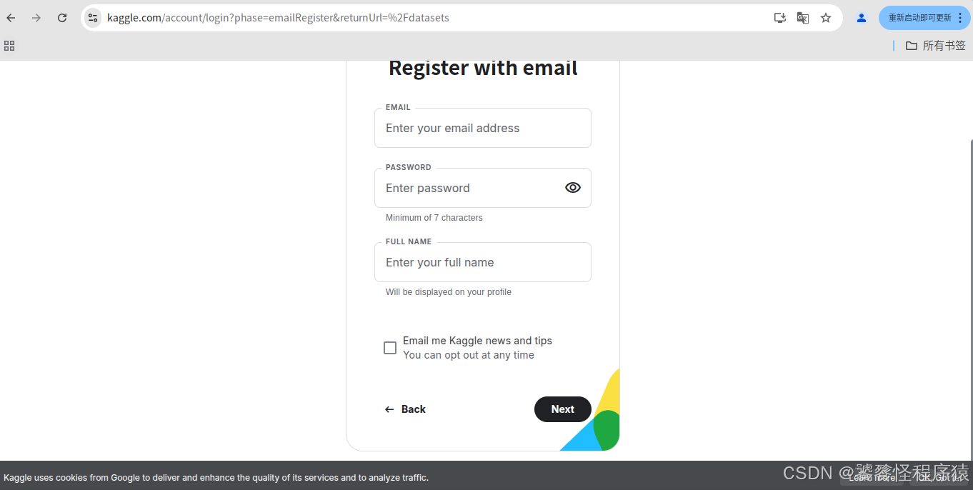
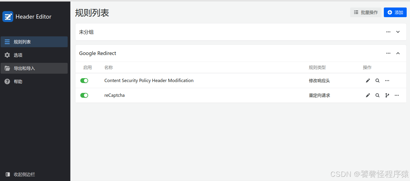
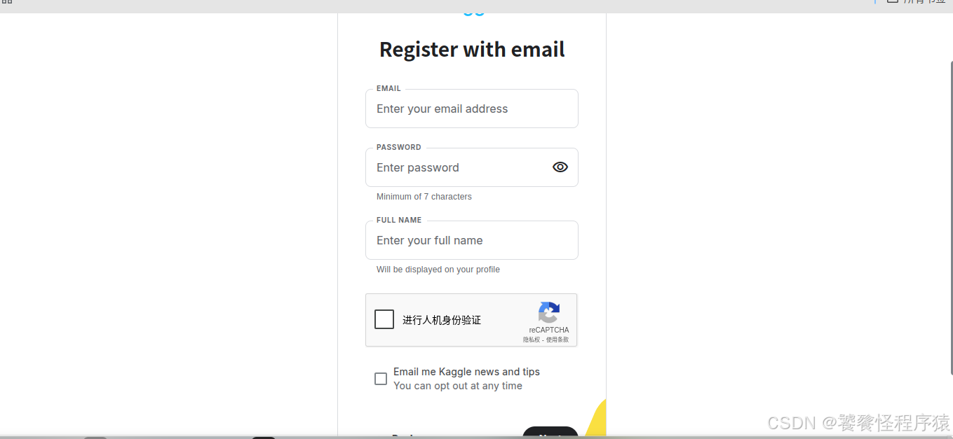
使用邮箱进行注册，但是通常会因为网络问题导致验证码无法正常显示，此时需要安装插件 Header Editor，将网页URL进行重定向，让验证码显示出来。

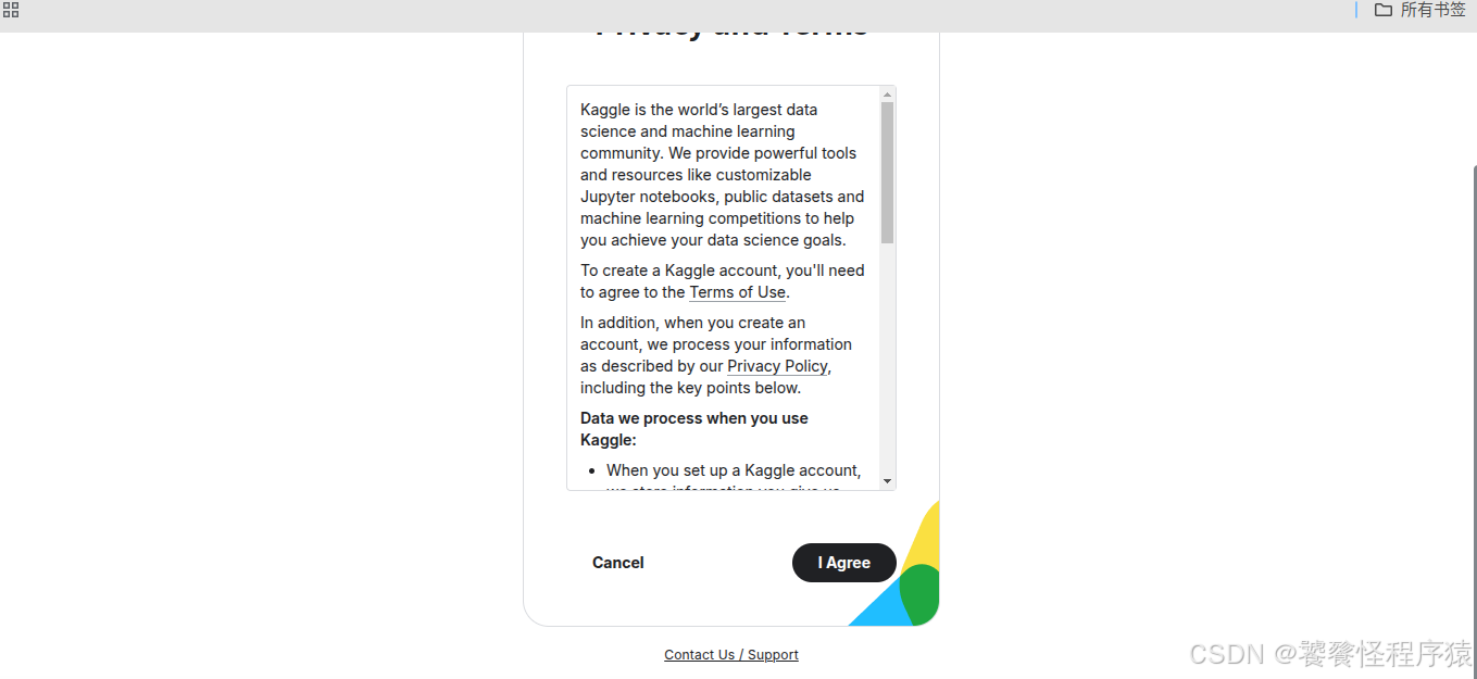
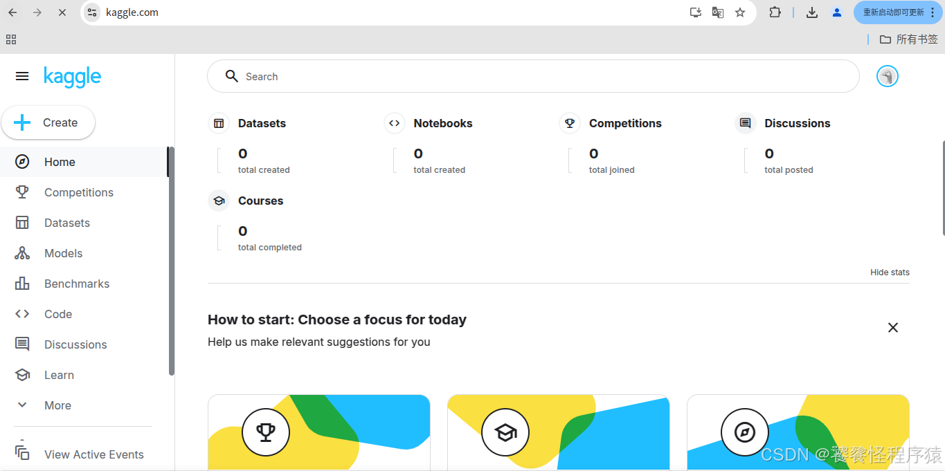
如图，到这里已经注册成功了。

二、竞赛入门

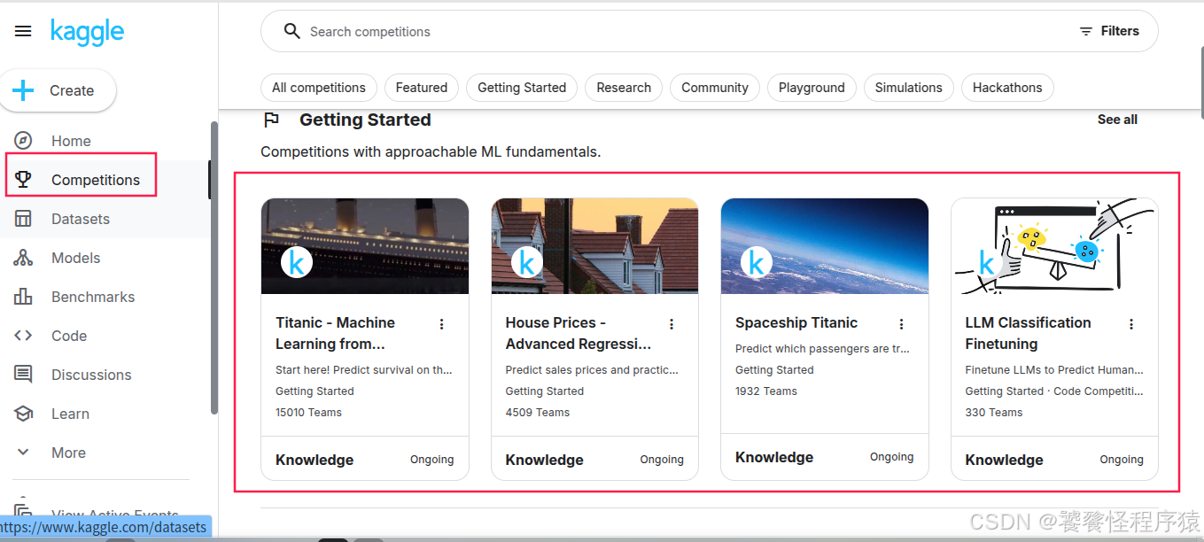
官方提供了一些入门级竞赛项目，非常容易上手，我们可以从这些赛事入手。

三、房价预测竞赛

例如，我们可以从 House Prices - Advanced Regression Techniques 这个赛事开始。

1、背景与任务

根据 Overview 页面的介绍，我们可以得知：购房者理想房屋描述与真实价格差异往往由多个因素决定，赛事提供了79个解释变量包含了住宅几乎各方面特征，希望参赛者能够使用这些特征进行最终房价预测。

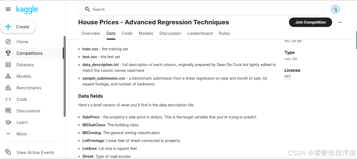
2、数据集

每个数据集的每个字段在 Data 页面都有具体说明：

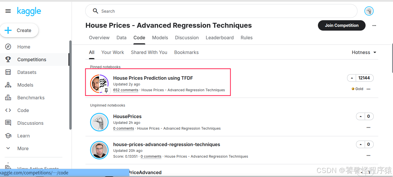
3、Baseline

在 Code 页面中，House Prices Prediction using TFDF 是一个能够完成赛事任务的基础实现方案，同时也可以看到众多参赛者分享的 Notebook：

四、跑通Baseline

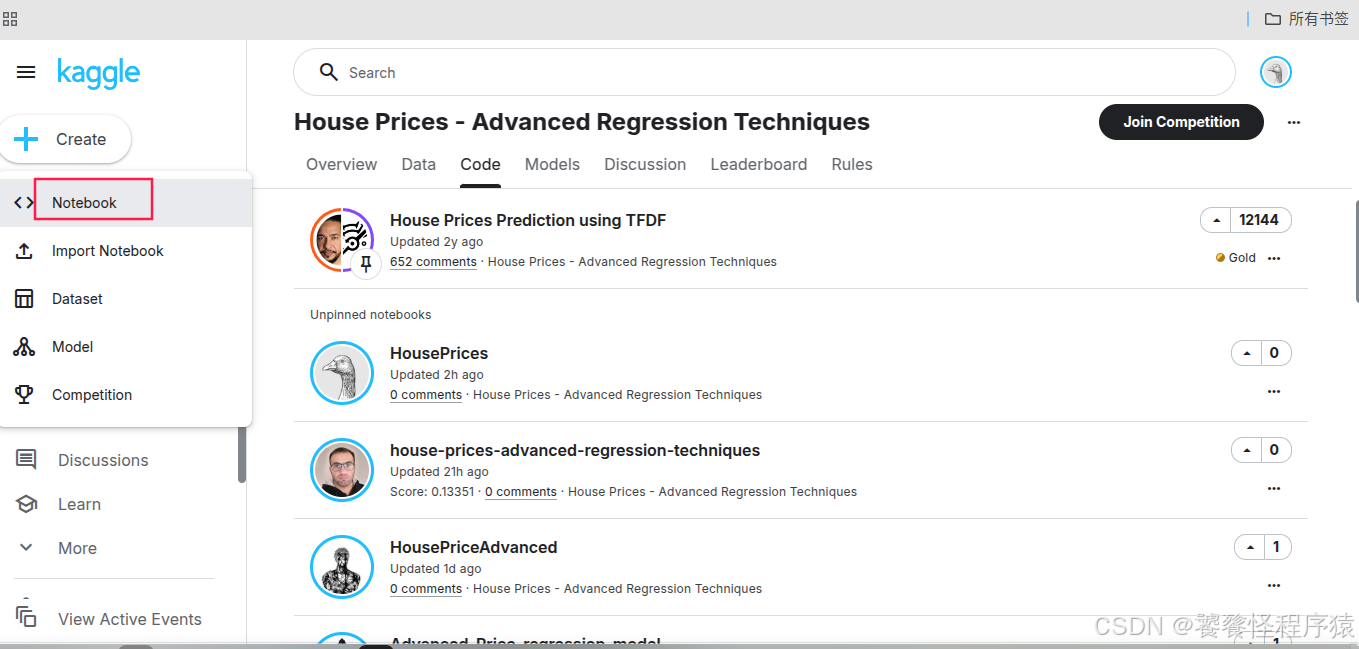
1、创建一个notebook

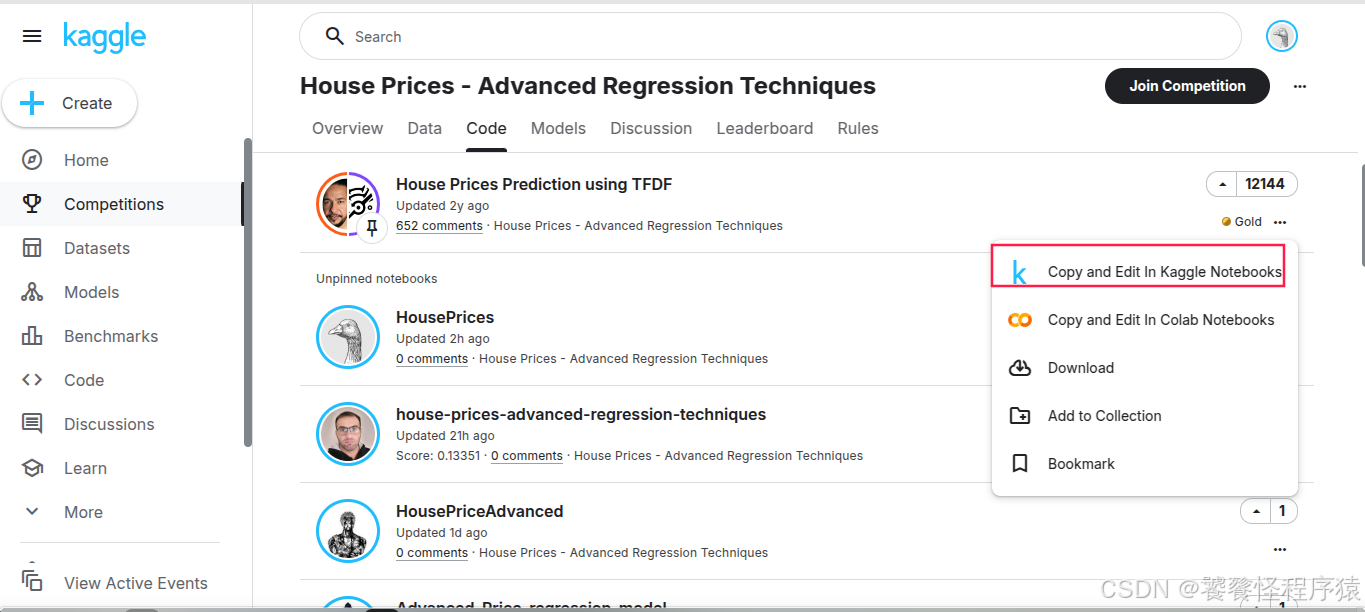
可以直接复制一份 Baseline 的 Notebook，也可以手动创建一个新的 Notebook：

为了方便演示，这里直接复制一份 Baseline：

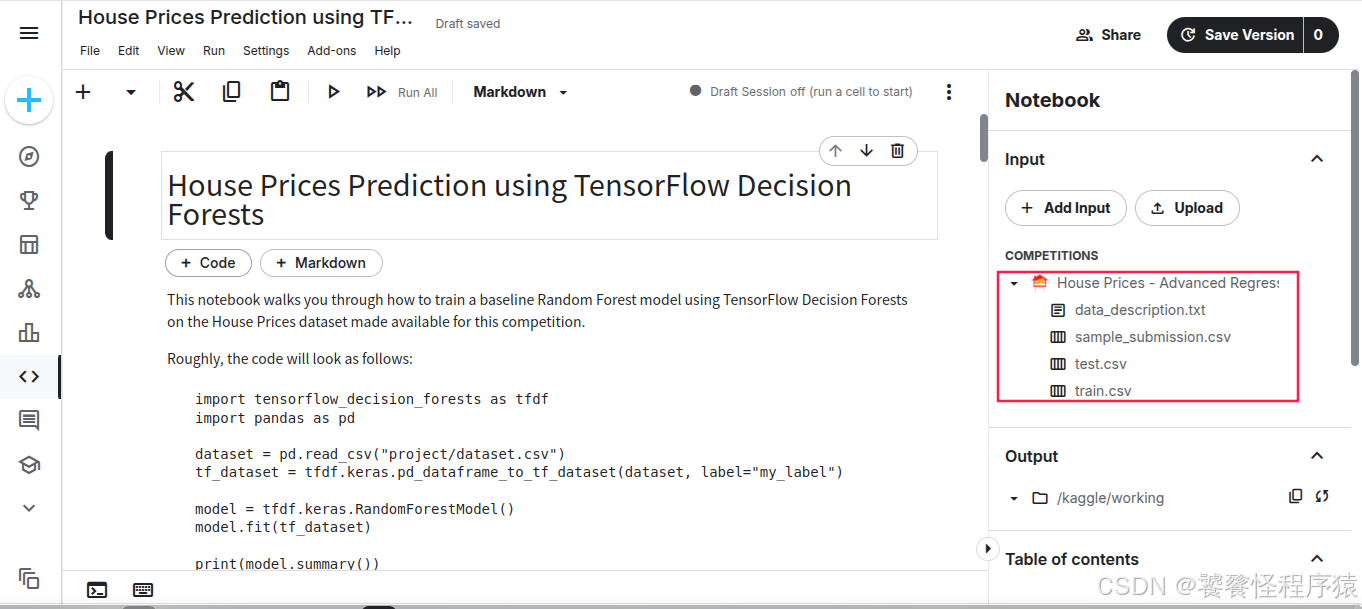
可以看到，该 Notebook 还自动引入了竞赛数据集，现在所有事情都可以在云端完成，无需本地搭建开发环境，非常方便。

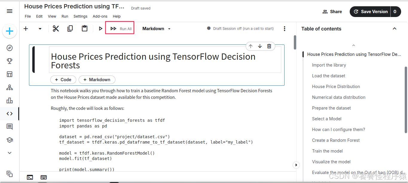
2、一键执行代码

3、提交预测结果

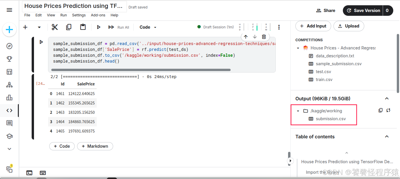
所有代码执行完毕之后，在 output 目录下生成 submission.csv 结果文件，该文件就是对房价进行预测后的结果文件。

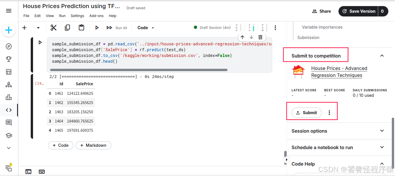
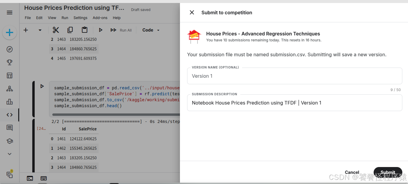
此时可以直接展开 Submit to competition 提交预测文件：

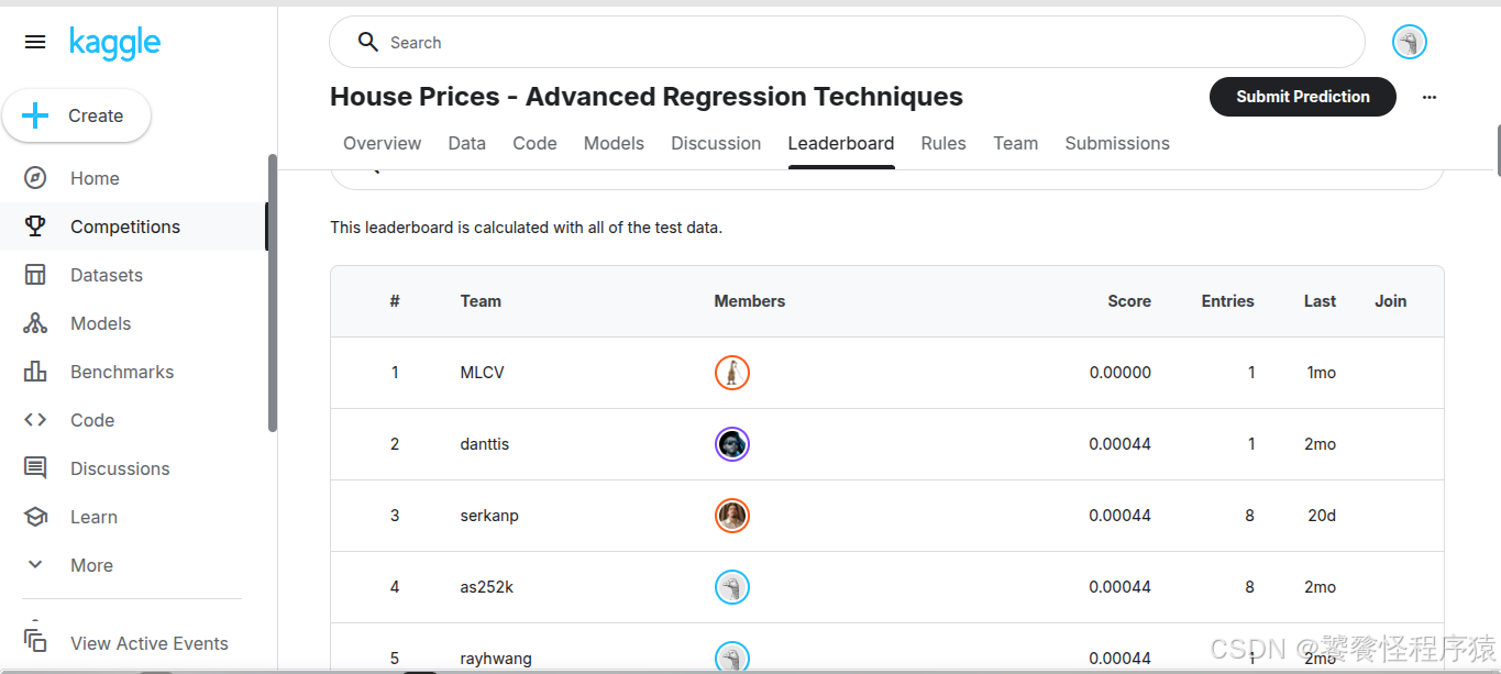
4、得分与排行榜

在赛事的 Leaderboard 页面可以查看自己的得分与名次：

五、Baseline拆解

Step1、导入依赖

import tensorflow as tf
import tensorflow_decision_forests as tfdf
import pandas as pd
import seaborn as sns
import matplotlib.pyplot as plt# Comment this if the data visualisations doesn't work on your side
%matplotlib inline

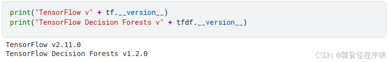
TensorFlow v2.11.0
TensorFlow Decision Forests v1.2.0

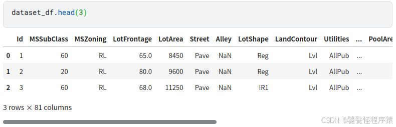
Step2、加载数据集

train_file_path = "../input/house-prices-advanced-regression-techniques/train.csv"
dataset_df = pd.read_csv(train_file_path)
print("Full train dataset shape is {}".format(dataset_df.shape))

Full train dataset shape is (1460, 81)

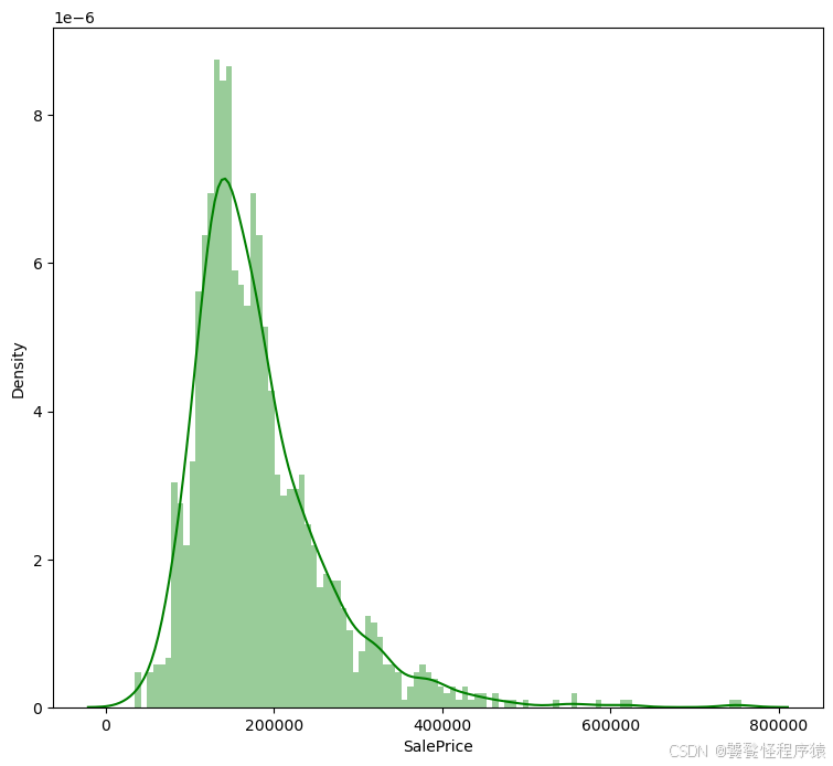
Step3、查看房价分布

print(dataset_df['SalePrice'].describe())
plt.figure(figsize=(9, 8))
sns.distplot(dataset_df['SalePrice'], color='g', bins=100, hist_kws={'alpha': 0.4});

count      1460.000000
mean     180921.195890
std       79442.502883
min       34900.000000
25%      129975.000000
50%      163000.000000
75%      214000.000000
max      755000.000000
Name: SalePrice, dtype: float64

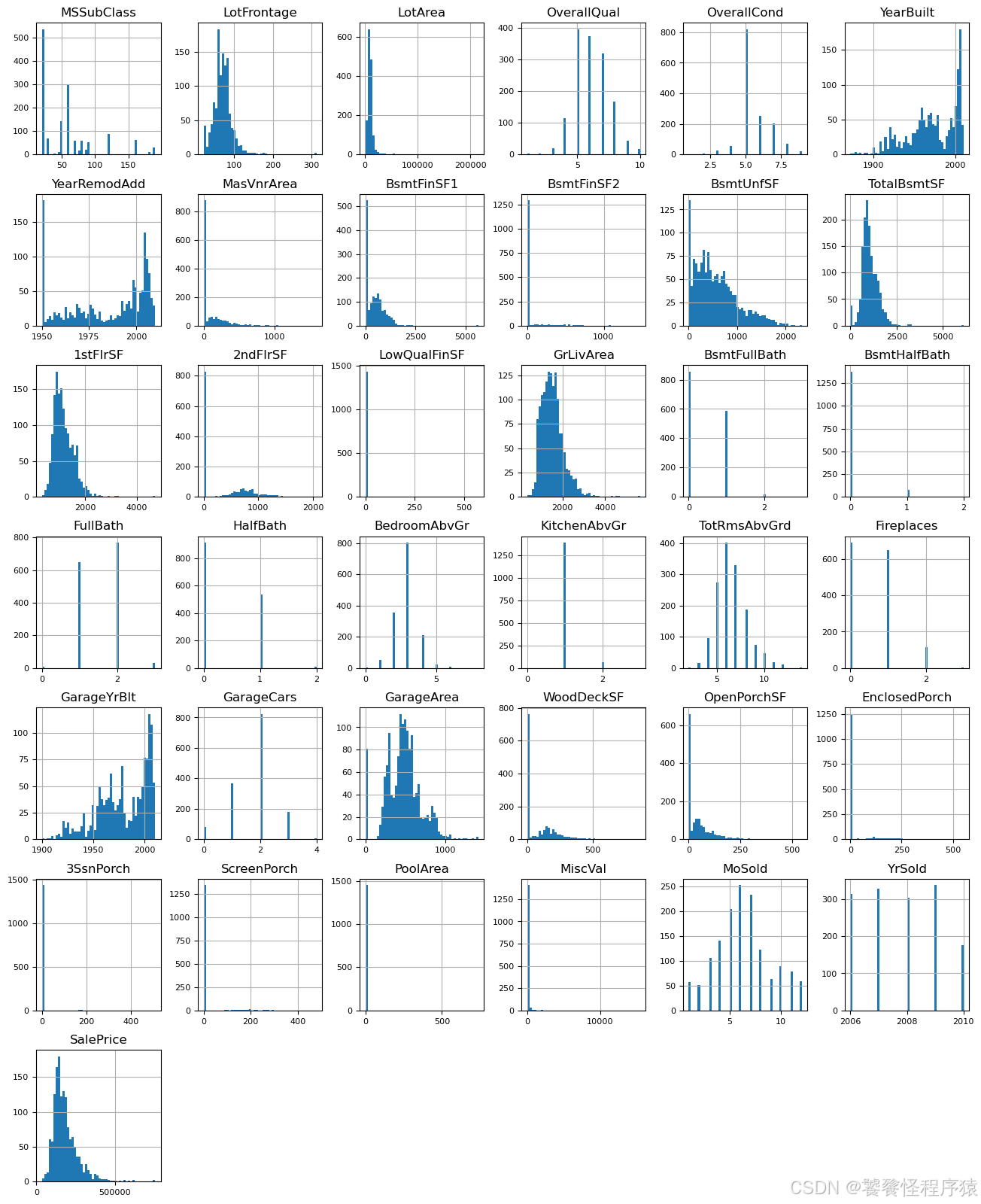
Step4、数值数据分布

list(set(dataset_df.dtypes.tolist()))df_num = dataset_df.select_dtypes(include = ['float64', 'int64'])
df_num.head()df_num.hist(figsize=(16, 20), bins=50, xlabelsize=8, ylabelsize=8);

Step5、划分数据集

import numpy as npdef split_dataset(dataset, test_ratio=0.30):test_indices = np.random.rand(len(dataset)) < test_ratioreturn dataset[~test_indices], dataset[test_indices]train_ds_pd, valid_ds_pd = split_dataset(dataset_df)
print("{} examples in training, {} examples in testing.".format(len(train_ds_pd), len(valid_ds_pd)))

label = 'SalePrice'
train_ds = tfdf.keras.pd_dataframe_to_tf_dataset(train_ds_pd, label=label, task = tfdf.keras.Task.REGRESSION)
valid_ds = tfdf.keras.pd_dataframe_to_tf_dataset(valid_ds_pd, label=label, task = tfdf.keras.Task.REGRESSION)

Step6、选择随机森林模型

rf = tfdf.keras.RandomForestModel(task = tfdf.keras.Task.REGRESSION)
rf.compile(metrics=["mse"]) # Optional, you can use this to include a list of eval metrics

Step7、训练模型

rf.fit(x=train_ds)

Step8、评估模型

import matplotlib.pyplot as plt
logs = rf.make_inspector().training_logs()
plt.plot([log.num_trees for log in logs], [log.evaluation.rmse for log in logs])
plt.xlabel("Number of trees")
plt.ylabel("RMSE (out-of-bag)")
plt.show()

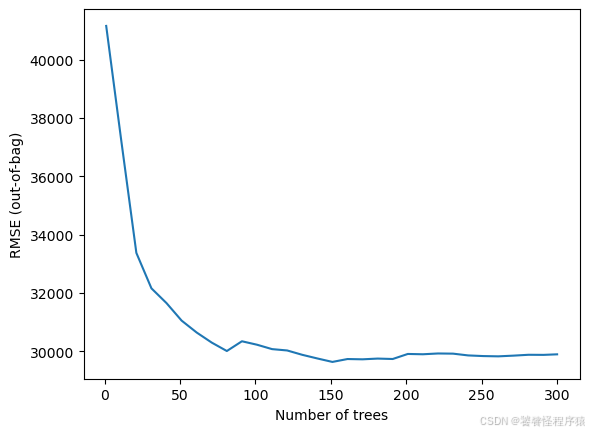
inspector = rf.make_inspector()
inspector.evaluation()

Evaluation(num_examples=1019, accuracy=None, loss=None, rmse=29893.939666232716, ndcg=None, aucs=None, auuc=None, qini=None)

evaluation = rf.evaluate(x=valid_ds,return_dict=True)for name, value in evaluation.items():print(f"{name}: {value:.4f}")

1/1 [==============================] - 1s 747ms/step - loss: 0.0000e+00 - mse: 698953728.0000
loss: 0.0000
mse: 698953728.0000

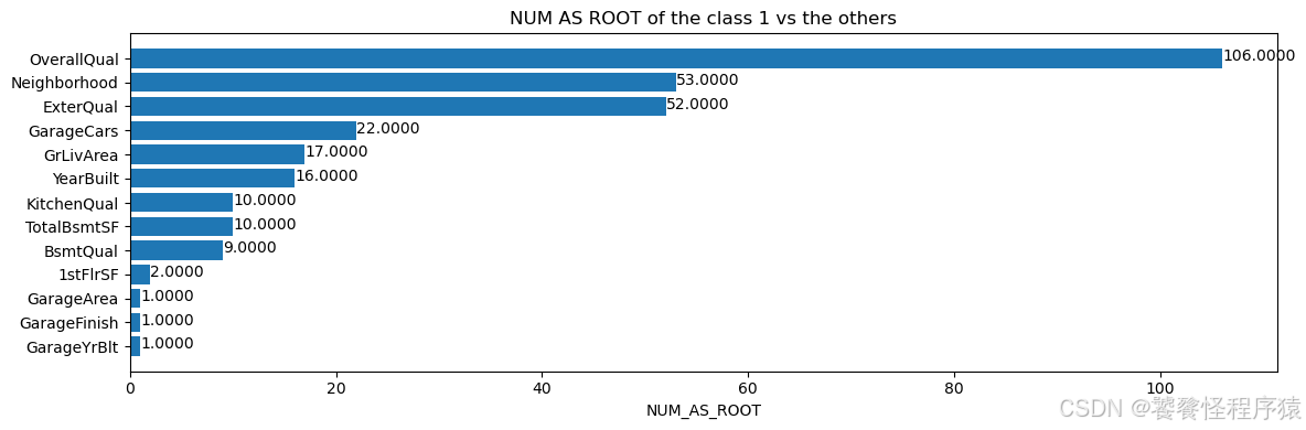
Step9、特征重要性

print(f"Available variable importances:")
for importance in inspector.variable_importances().keys():print("\t", importance)

Available variable importances:SUM_SCORENUM_AS_ROOTNUM_NODESINV_MEAN_MIN_DEPTH

inspector.variable_importances()["NUM_AS_ROOT"]

[("OverallQual" (1; #62), 106.0),("Neighborhood" (4; #59), 53.0),("ExterQual" (4; #22), 52.0),("GarageCars" (1; #32), 22.0),("GrLivArea" (1; #38), 17.0),("YearBuilt" (1; #76), 16.0),("KitchenQual" (4; #44), 10.0),("TotalBsmtSF" (1; #73), 10.0),("BsmtQual" (4; #14), 9.0),("1stFlrSF" (1; #0), 2.0),("GarageArea" (1; #31), 1.0),("GarageFinish" (4; #34), 1.0),("GarageYrBlt" (1; #37), 1.0)]

plt.figure(figsize=(12, 4))# Mean decrease in AUC of the class 1 vs the others.
variable_importance_metric = "NUM_AS_ROOT"
variable_importances = inspector.variable_importances()[variable_importance_metric]# Extract the feature name and importance values.
#
# `variable_importances` is a list of <feature, importance> tuples.
feature_names = [vi[0].name for vi in variable_importances]
feature_importances = [vi[1] for vi in variable_importances]
# The feature are ordered in decreasing importance value.
feature_ranks = range(len(feature_names))bar = plt.barh(feature_ranks, feature_importances, label=[str(x) for x in feature_ranks])
plt.yticks(feature_ranks, feature_names)
plt.gca().invert_yaxis()# TODO: Replace with "plt.bar_label()" when available.
# Label each bar with values
for importance, patch in zip(feature_importances, bar.patches):plt.text(patch.get_x() + patch.get_width(), patch.get_y(), f"{importance:.4f}", va="top")plt.xlabel(variable_importance_metric)
plt.title("NUM AS ROOT of the class 1 vs the others")
plt.tight_layout()
plt.show()

Step10、保存预测结果

test_file_path = "../input/house-prices-advanced-regression-techniques/test.csv"
test_data = pd.read_csv(test_file_path)
ids = test_data.pop('Id')test_ds = tfdf.keras.pd_dataframe_to_tf_dataset(test_data,task = tfdf.keras.Task.REGRESSION)preds = rf.predict(test_ds)
output = pd.DataFrame({'Id': ids,'SalePrice': preds.squeeze()})output.head()

sample_submission_df = pd.read_csv('../input/house-prices-advanced-regression-techniques/sample_submission.csv')
sample_submission_df['SalePrice'] = rf.predict(test_ds)
sample_submission_df.to_csv('/kaggle/working/submission.csv', index=False)
sample_submission_df.head()

Next Steps

微调模型，上分打榜。