深度学习笔记39-CGAN｜生成手势图像 | 可控制生成(Pytorch)

•  🍨 本文为🔗365天深度学习训练营中的学习记录博客
• 🍖 原作者：K同学啊

一、概念

条件生成对抗网络（CGAN）是在生成对抗网络（GAN）的基础上进行了一些改进。对于原始GAN的生成器而言，其生成的图像数据是随机不可预测的，因此我们无法控制网络的输出，在实际操作中的可控性不强。

        针对上述原始GAN无法生成具有特定属性的图像数据的问题，Mehdi Mirza等人在2014年提出了条件生成对抗网络，通过给原始生成对抗网络中的生成器G和判别器D增加额外的条件，例如我们需要生成器G生成一张没有阴影的图像，此时判别器D就需要判断生成器所生成的图像是否是一张没有阴影的图像。条件生成对抗网络的本质是将额外添加的信息融入到生成器和判别器中，其中添加的信息可以是图像的类别、人脸表情和其他辅助信息等，旨在把无监督学习的GAN转化为有监督学习的CGAN，便于网络能够在我们的掌控下更好地进行训练。CGAN网络结构如下图所示。

​

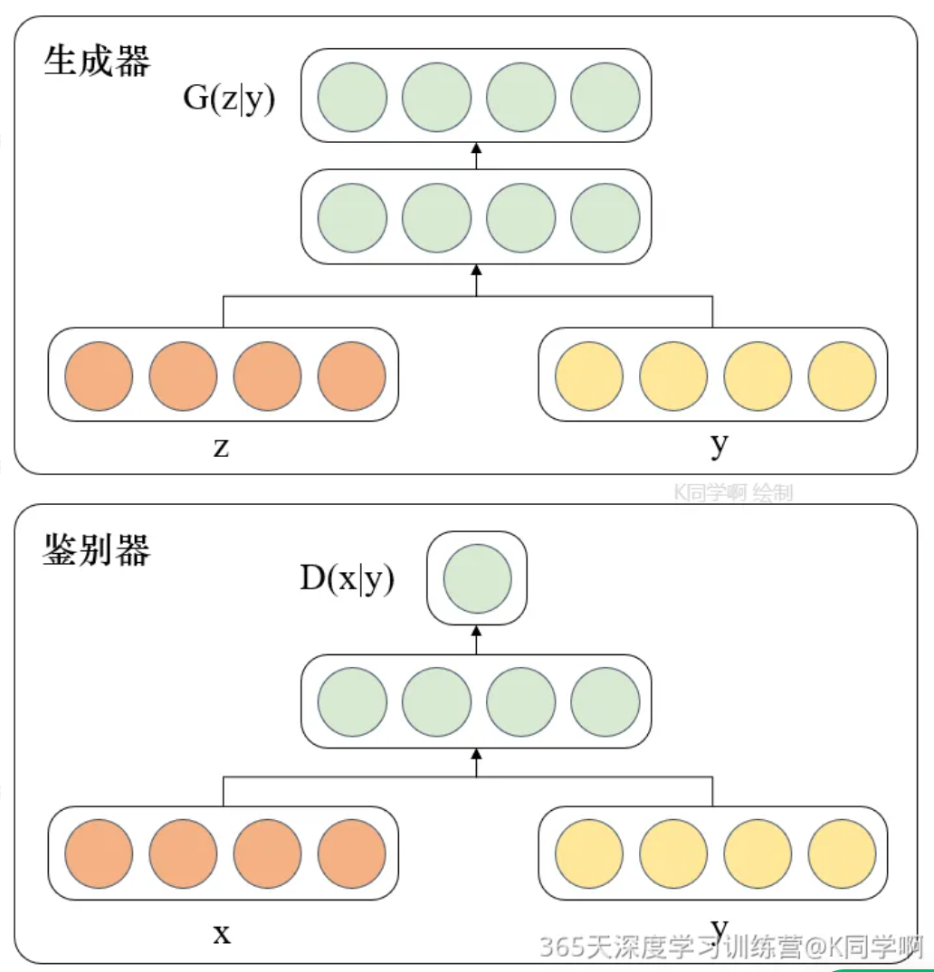
由网络结构可知，条件信息y作为额外的输入被引入对抗网络中，与生成器中的噪声z合并作为隐含层表达;而在判别器D中，条件信息y则与原始数据x合并作为判别函数的输入。这种改进在以后的诸多方面研究中被证明是非常有效的，也为后续的相关工作提供了积极的指导作用。

二、前期工作

1.导入数据及可视化

from torchvision       import datasets, transforms
from torch.autograd    import Variable
from torchvision.utils import save_image, make_grid
from torchsummary      import summary
import matplotlib.pyplot as plt
import numpy             as np
import torch.nn          as nn
import torch.optim       as optim
import torchdevice = torch.device('cuda' if torch.cuda.is_available() else 'cpu')
devicebatch_size = 128train_transform = transforms.Compose([transforms.Resize(128),transforms.ToTensor(),transforms.Normalize([0.5,0.5,0.5], [0.5,0.5,0.5])])train_dataset = datasets.ImageFolder(root='data/data/rps/', transform=train_transform)train_loader = torch.utils.data.DataLoader(dataset=train_dataset, batch_size=batch_size, shuffle=True,num_workers=6)# 可视化第一个 batch 的数据
def show_images(dl):for images, _ in dl:fig, ax = plt.subplots(figsize=(10, 10))ax.set_xticks([]); ax.set_yticks([])ax.imshow(make_grid(images.detach(), nrow=16).permute(1, 2, 0))breakshow_images(train_loader)

2.构建模型

latent_dim    = 100
n_classes     = 3
embedding_dim = 100# 自定义权重初始化函数，用于初始化生成器和判别器的权重
def weights_init(m):# 获取当前层的类名classname = m.__class__.__name__# 如果当前层是卷积层（类名中包含 'Conv' ）if classname.find('Conv') != -1:# 使用正态分布随机初始化权重，均值为0，标准差为0.02torch.nn.init.normal_(m.weight, 0.0, 0.02)# 如果当前层是批归一化层（类名中包含 'BatchNorm' ）elif classname.find('BatchNorm') != -1:# 使用正态分布随机初始化权重，均值为1，标准差为0.02torch.nn.init.normal_(m.weight, 1.0, 0.02)# 将偏置项初始化为全零torch.nn.init.zeros_(m.bias)class Generator(nn.Module):def __init__(self):super(Generator, self).__init__()# 定义条件标签的生成器部分，用于将标签映射到嵌入空间中# n_classes：条件标签的总数# embedding_dim：嵌入空间的维度self.label_conditioned_generator = nn.Sequential(nn.Embedding(n_classes, embedding_dim),  # 使用Embedding层将条件标签映射为稠密向量nn.Linear(embedding_dim, 16)             # 使用线性层将稠密向量转换为更高维度)# 定义潜在向量的生成器部分，用于将噪声向量映射到图像空间中# latent_dim：潜在向量的维度self.latent = nn.Sequential(nn.Linear(latent_dim, 4*4*512),  # 使用线性层将潜在向量转换为更高维度nn.LeakyReLU(0.2, inplace=True)  # 使用LeakyReLU激活函数进行非线性映射)# 定义生成器的主要结构，将条件标签和潜在向量合并成生成的图像self.model = nn.Sequential(# 反卷积层1：将合并后的向量映射为64x8x8的特征图nn.ConvTranspose2d(513, 64*8, 4, 2, 1, bias=False),nn.BatchNorm2d(64*8, momentum=0.1, eps=0.8),  # 批标准化nn.ReLU(True),  # ReLU激活函数# 反卷积层2：将64x8x8的特征图映射为64x4x4的特征图nn.ConvTranspose2d(64*8, 64*4, 4, 2, 1, bias=False),nn.BatchNorm2d(64*4, momentum=0.1, eps=0.8),nn.ReLU(True),# 反卷积层3：将64x4x4的特征图映射为64x2x2的特征图nn.ConvTranspose2d(64*4, 64*2, 4, 2, 1, bias=False),nn.BatchNorm2d(64*2, momentum=0.1, eps=0.8),nn.ReLU(True),# 反卷积层4：将64x2x2的特征图映射为64x1x1的特征图nn.ConvTranspose2d(64*2, 64*1, 4, 2, 1, bias=False),nn.BatchNorm2d(64*1, momentum=0.1, eps=0.8),nn.ReLU(True),# 反卷积层5：将64x1x1的特征图映射为3x64x64的RGB图像nn.ConvTranspose2d(64*1, 3, 4, 2, 1, bias=False),nn.Tanh()  # 使用Tanh激活函数将生成的图像像素值映射到[-1, 1]范围内)def forward(self, inputs):noise_vector, label = inputs# 通过条件标签生成器将标签映射为嵌入向量label_output = self.label_conditioned_generator(label)# 将嵌入向量的形状变为（batch_size, 1, 4, 4），以便与潜在向量进行合并label_output = label_output.view(-1, 1, 4, 4)# 通过潜在向量生成器将噪声向量映射为潜在向量latent_output = self.latent(noise_vector)# 将潜在向量的形状变为（batch_size, 512, 4, 4），以便与条件标签进行合并latent_output = latent_output.view(-1, 512, 4, 4)# 将条件标签和潜在向量在通道维度上进行合并，得到合并后的特征图concat = torch.cat((latent_output, label_output), dim=1)# 通过生成器的主要结构将合并后的特征图生成为RGB图像image = self.model(concat)return image
generator = Generator().to(device)
generator.apply(weights_init)
print(generator)from torchinfo import summarysummary(generator)a = torch.ones(100)
b = torch.ones(1)
b = b.long()
a = a.to(device)
b = b.to(device)import torch
import torch.nn as nnclass Discriminator(nn.Module):def __init__(self):super(Discriminator, self).__init__()# 定义一个条件标签的嵌入层，用于将类别标签转换为特征向量self.label_condition_disc = nn.Sequential(nn.Embedding(n_classes, embedding_dim),     # 嵌入层将类别标签编码为固定长度的向量nn.Linear(embedding_dim, 3*128*128)         # 线性层将嵌入的向量转换为与图像尺寸相匹配的特征张量)# 定义主要的鉴别器模型self.model = nn.Sequential(nn.Conv2d(6, 64, 4, 2, 1, bias=False),       # 输入通道为6（包含图像和标签的通道数），输出通道为64，4x4的卷积核，步长为2，padding为1nn.LeakyReLU(0.2, inplace=True),             # LeakyReLU激活函数，带有负斜率，增加模型对输入中的负值的感知能力nn.Conv2d(64, 64*2, 4, 3, 2, bias=False),    # 输入通道为64，输出通道为64*2，4x4的卷积核，步长为3，padding为2nn.BatchNorm2d(64*2, momentum=0.1, eps=0.8),  # 批量归一化层，有利于训练稳定性和收敛速度nn.LeakyReLU(0.2, inplace=True),nn.Conv2d(64*2, 64*4, 4, 3, 2, bias=False),  # 输入通道为64*2，输出通道为64*4，4x4的卷积核，步长为3，padding为2nn.BatchNorm2d(64*4, momentum=0.1, eps=0.8),nn.LeakyReLU(0.2, inplace=True),nn.Conv2d(64*4, 64*8, 4, 3, 2, bias=False),  # 输入通道为64*4，输出通道为64*8，4x4的卷积核，步长为3，padding为2nn.BatchNorm2d(64*8, momentum=0.1, eps=0.8),nn.LeakyReLU(0.2, inplace=True),nn.Flatten(),                               # 将特征图展平为一维向量，用于后续全连接层处理nn.Dropout(0.4),                            # 随机失活层，用于减少过拟合风险nn.Linear(4608, 1),                         # 全连接层，将特征向量映射到输出维度为1的向量nn.Sigmoid()                                # Sigmoid激活函数，用于输出范围限制在0到1之间的概率值)def forward(self, inputs):img, label = inputs# 将类别标签转换为特征向量label_output = self.label_condition_disc(label)# 重塑特征向量为与图像尺寸相匹配的特征张量label_output = label_output.view(-1, 3, 128, 128)# 将图像特征和标签特征拼接在一起作为鉴别器的输入concat = torch.cat((img, label_output), dim=1)# 将拼接后的输入通过鉴别器模型进行前向传播，得到输出结果output = self.model(concat)return outputdiscriminator = Discriminator().to(device)
discriminator.apply(weights_init)
print(discriminator)summary(discriminator)a = torch.ones(2,3,128,128)
b = torch.ones(2,1)
b = b.long()
a = a.to(device)
b = b.to(device)c = discriminator((a,b))
c.size()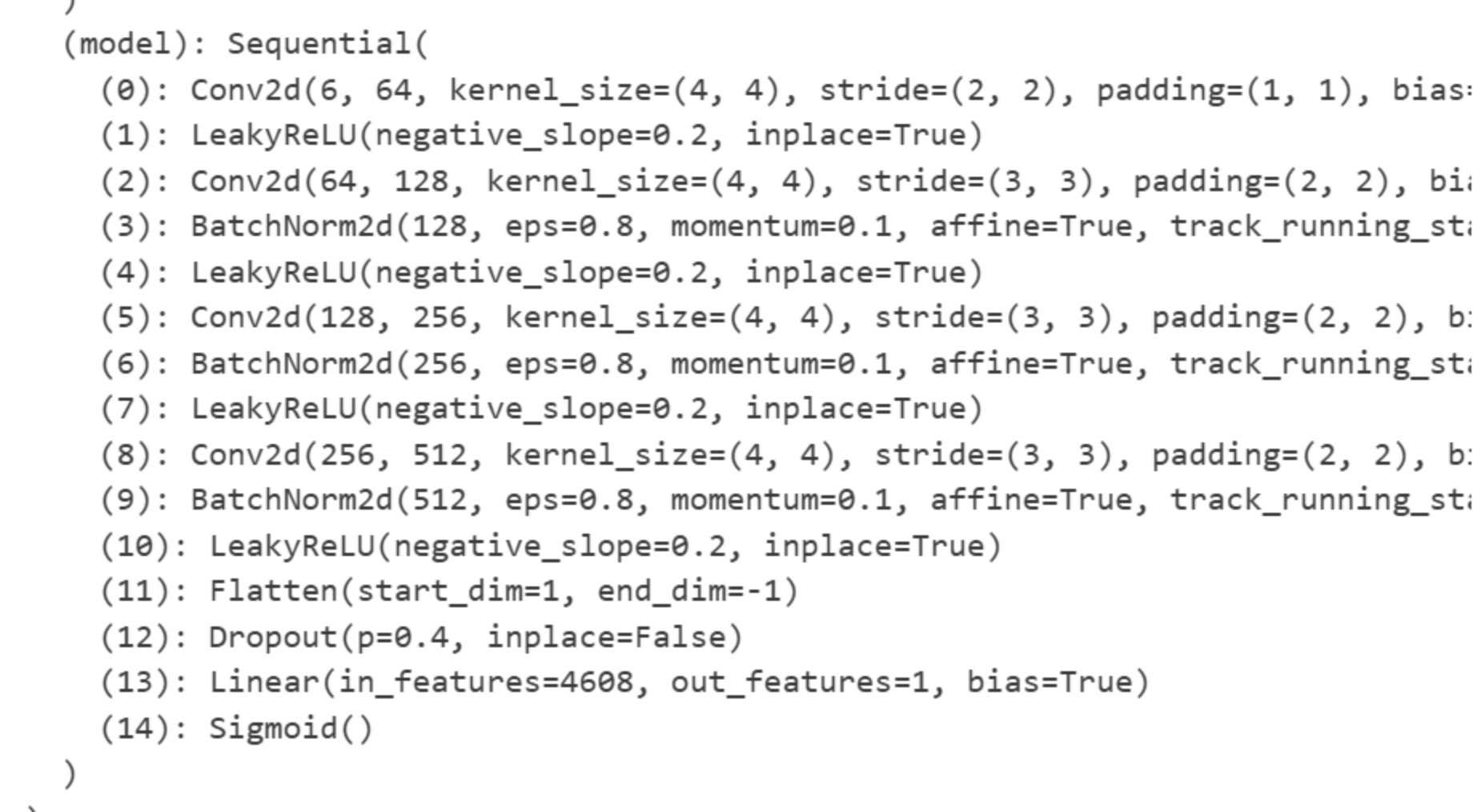

​

3.训练模型

adversarial_loss = nn.BCELoss() def generator_loss(fake_output, label):gen_loss = adversarial_loss(fake_output, label)return gen_lossdef discriminator_loss(output, label):disc_loss = adversarial_loss(output, label)return disc_losslearning_rate = 0.0002G_optimizer = optim.Adam(generator.parameters(),     lr = learning_rate, betas=(0.5, 0.999))
D_optimizer = optim.Adam(discriminator.parameters(), lr = learning_rate, betas=(0.5, 0.999))# 设置训练的总轮数
num_epochs = 300
# 初始化用于存储每轮训练中判别器和生成器损失的列表
D_loss_plot, G_loss_plot = [], []# 循环进行训练
for epoch in range(1, num_epochs + 1):# 初始化每轮训练中判别器和生成器损失的临时列表D_loss_list, G_loss_list = [], []# 遍历训练数据加载器中的数据for index, (real_images, labels) in enumerate(train_loader):# 清空判别器的梯度缓存D_optimizer.zero_grad()# 将真实图像数据和标签转移到GPU（如果可用）real_images = real_images.to(device)labels      = labels.to(device)# 将标签的形状从一维向量转换为二维张量（用于后续计算）labels = labels.unsqueeze(1).long()# 创建真实目标和虚假目标的张量（用于判别器损失函数）real_target = Variable(torch.ones(real_images.size(0), 1).to(device))fake_target = Variable(torch.zeros(real_images.size(0), 1).to(device))# 计算判别器对真实图像的损失D_real_loss = discriminator_loss(discriminator((real_images, labels)), real_target)# 从噪声向量中生成假图像（生成器的输入）noise_vector = torch.randn(real_images.size(0), latent_dim, device=device)noise_vector = noise_vector.to(device)generated_image = generator((noise_vector, labels))# 计算判别器对假图像的损失（注意detach()函数用于分离生成器梯度计算图）output = discriminator((generated_image.detach(), labels))D_fake_loss = discriminator_loss(output, fake_target)# 计算判别器总体损失（真实图像损失和假图像损失的平均值）D_total_loss = (D_real_loss + D_fake_loss) / 2D_loss_list.append(D_total_loss.item())# 反向传播更新判别器的参数D_total_loss.backward()D_optimizer.step()# 清空生成器的梯度缓存G_optimizer.zero_grad()# 计算生成器的损失G_loss = generator_loss(discriminator((generated_image, labels)), real_target)G_loss_list.append(G_loss.item())# 反向传播更新生成器的参数G_loss.backward()G_optimizer.step()# 打印当前轮次的判别器和生成器的平均损失print('Epoch: [%d/%d]: D_loss: %.3f, G_loss: %.3f' % ((epoch), num_epochs, torch.mean(torch.FloatTensor(D_loss_list)), torch.mean(torch.FloatTensor(G_loss_list))))# 将当前轮次的判别器和生成器的平均损失保存到列表中D_loss_plot.append(torch.mean(torch.FloatTensor(D_loss_list)))G_loss_plot.append(torch.mean(torch.FloatTensor(G_loss_list)))if epoch%10 == 0:# 将生成的假图像保存为图片文件save_image(generated_image.data[:50], './images/sample_%d' % epoch + '.png', nrow=5, normalize=True)# 将当前轮次的生成器和判别器的权重保存到文件torch.save(generator.state_dict(), './training_weights/generator_epoch_%d.pth' % (epoch))torch.save(discriminator.state_dict(), './training_weights/discriminator_epoch_%d.pth' % (epoch))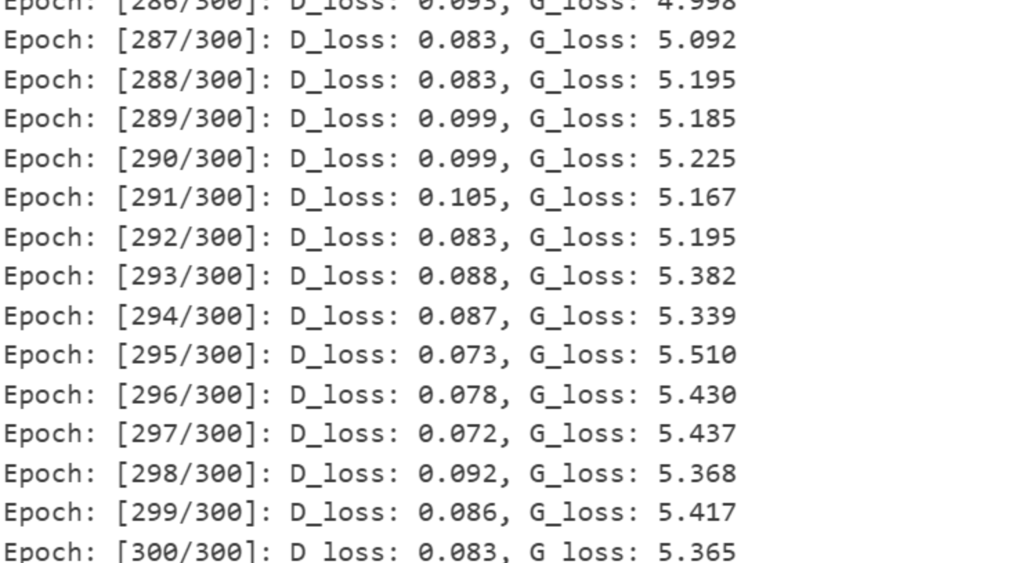

​

4.生成指定图像

G_loss_list = [i.item() for i in G_loss_plot]
D_loss_list = [i.item() for i in D_loss_plot]import matplotlib.pyplot as plt
#隐藏警告
import warnings
warnings.filterwarnings("ignore")               #忽略警告信息
plt.rcParams['font.sans-serif']    = ['SimHei'] # 用来正常显示中文标签
plt.rcParams['axes.unicode_minus'] = False      # 用来正常显示负号
plt.rcParams['figure.dpi']         = 100        #分辨率plt.figure(figsize=(8,4))
plt.title("Generator and Discriminator Loss During Training")
plt.plot(G_loss_list,label="G")
plt.plot(D_loss_list,label="D")
plt.xlabel("iterations")
plt.ylabel("Loss")
plt.legend()
plt.show()# 导入所需的库
from numpy.random import randint, randn
from numpy        import linspace
from matplotlib   import pyplot, gridspec# 导入生成器模型
generator.load_state_dict(torch.load('./training_weights/generator_epoch_300.pth'), strict=False)
generator.eval()   interpolated = randn(100)  # 生成两个潜在空间的点
# 将数据转换为torch张量并将其移至GPU（假设device已正确声明为GPU）
interpolated = torch.tensor(interpolated).to(device).type(torch.float32)label  = 0  # 手势标签，可在0,1,2之间选择
labels = torch.ones(1) * label
labels = labels.to(device).unsqueeze(1).long()# 使用生成器生成插值结果
predictions = generator((interpolated, labels))
predictions = predictions.permute(0,2,3,1).detach().cpu()#隐藏警告
import warnings
warnings.filterwarnings("ignore")               #忽略警告信息
plt.rcParams['font.sans-serif']    = ['SimHei'] # 用来正常显示中文标签
plt.rcParams['axes.unicode_minus'] = False      # 用来正常显示负号
plt.rcParams['figure.dpi']         = 100        #分辨率plt.figure(figsize=(8, 3))pred = (predictions[0, :, :, :] + 1 ) * 127.5
pred = np.array(pred)
plt.imshow(pred.astype(np.uint8))
plt.show()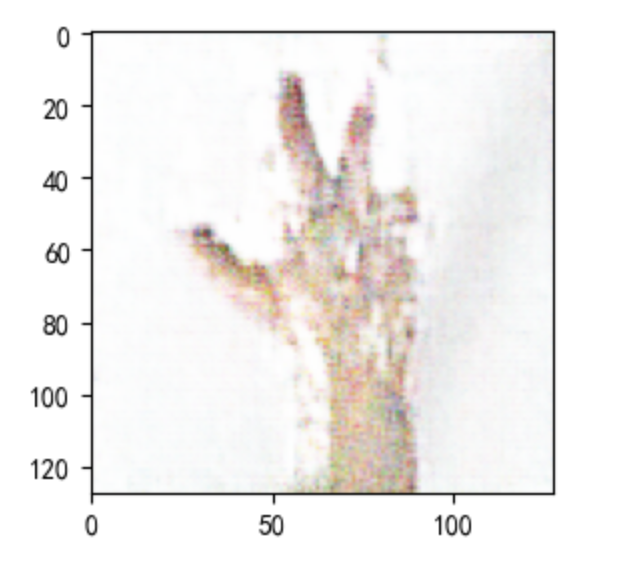

​

三、总结

数据集: 使用了torchvision.datasets.ImageFolder加载自定义的图像文件夹，并对图像进行了变换，包括调整大小、转为张量以及归一化处理。
可视化: 通过show_images函数展示了训练集中第一个batch的数据，帮助理解输入数据的形态。
模型构建

• Generator (生成器): 构建了一个能够接收潜在向量和类别标签作为输入的生成器。通过嵌入层将类别标签转换为特征向量，并与潜在向量结合，然后经过一系列反卷积层生成目标图像。
• Discriminator (判别器): 构建了一个能够接收图像和类别标签作为输入的判别器。首先将类别标签转换为特征图并与输入图像结合，接着通过多个卷积层提取特征，最后输出一个标量值来判断输入图像的真实性。
• 权重初始化: 自定义了权重初始化方法weights_init，以确保模型中各层的权重初始分布有利于训练。

训练过程

• 损失函数: 使用了二元交叉熵损失BCELoss来计算生成器和判别器的损失。
• 优化器: 使用Adam优化算法分别更新生成器和判别器的参数。
• 训练循环: 在每个epoch中，交替更新判别器和生成器的参数。对于每个batch的数据，先更新判别器，使其能够更好地分辨真实图像和生成图像；然后更新生成器，使其生成的图像更难以被判别器识别为假。
• 结果保存: 每隔10个epoch保存一次生成的图像样本和模型权重，以便于后续分析和模型恢复。

结果分析
通过记录每轮次的生成器和判别器损失，可以观察到模型训练的进展和收敛情况。随着训练的进行，生成器试图欺骗判别器，而判别器则努力区分真假图像，两者之间的竞争推动了模型性能的提升。