Information theorem-Entropy

Self -information
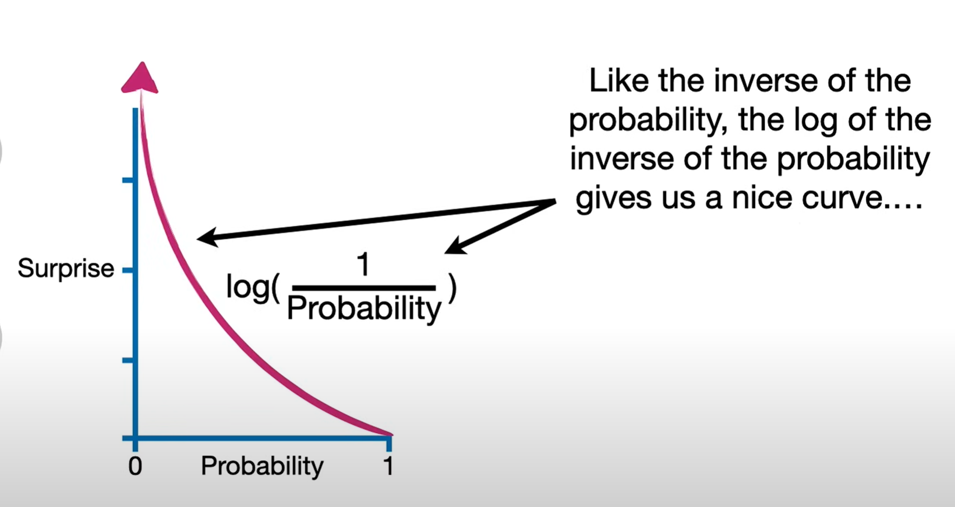
In information theory and statistics, “surprise” is quantified by self-information. For an event x with probability p(x), the amount of surprise (also called information content) is defined as
I(x)=−logp(x)=log1p(x).I(x) = -\log p(x)=\log \frac{1}{p(x)}.I(x)=−logp(x)=logp(x)1.
This definition has several nice properties:
-
Rarity gives more surprise: If p(x) is small, then I(x) is large — rare events are more surprising.
-
Certainty gives no surprise: If p(x)=1, then I(x)=0. Something guaranteed to happen is not surprising at all.
-
Additivity for independence: If two independent events occur, the total surprise is the sum of their individual surprises: I(x,y)=I(x)+I(y)
The logarithm base just changes the unit:base 2 gives “bits,” base e gives “nats.”
For example, if an event has probability 1/8, then
I(x)=−log218=3 bitsI(x) = -\log_2 \tfrac{1}{8} = 3 \ \text{bits}I(x)=−log281=3 bits
meaning the event carries 3 bits of surprise.
Entropy
Formally, entropy is defined as the expected surprise (expected self-information) under a probability distribution. For a random variable X with distribution p(x):
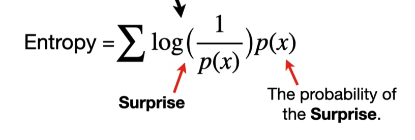
H(X)=E[I(X)]=∑xp(x) (−logp(x))=−∑xp(x)logp(x).H(X) = \mathbb{E}[I(X)] = \sum_{x} p(x)\,(-\log p(x)) = -\sum_{x} p(x)\log p(x).H(X)=E[I(X)]=x∑p(x)(−logp(x))=−x∑p(x)logp(x).
Key points:
-
Each outcome x carries a “surprise” I(x)=−logp(x)I(x) = -\log p(x)I(x)=−logp(x).
-
We weight that surprise by how likely it is p(x).
-
The entropy is the average surprise if you repeatedly observe X.
For example:
-
A fair coin (p(H)=p(T)=0.5p(H)=p(T)=0.5p(H)=p(T)=0.5) has
H=−[0.5log20.5+0.5log20.5]=1 bit.H = -[0.5\log_2 0.5 + 0.5\log_2 0.5] = 1 \text{ bit}.H=−[0.5log20.5+0.5log20.5]=1 bit.
Meaning: on average, each coin flip carries 1 bit of surprise.
-
A biased coin (p(H)=0.9,p(T)=0.1p(H)=0.9, p(T)=0.1p(H)=0.9,p(T)=0.1) has
H=−[0.9log20.9+0.1log20.1]≈0.47 bits.H = -[0.9\log_2 0.9 + 0.1\log_2 0.1] \approx 0.47 \text{ bits}.H=−[0.9log20.9+0.1log20.1]≈0.47 bits.
Less uncertainty → less average surprise.
So entropy = expected surprised amount you’d feel per observation, given your model.
Cross-entropy
H(P,Q)=−∑xp(x)logq(x)H(P,Q)=−∑_{x}p(x)logq(x)H(P,Q)=−x∑p(x)logq(x)
-
The weighting comes from the true distribution P (because that’s what actually happens in the world).
-
The surprise calculation −logq(x)−logq(x)−logq(x)comes from the model Q (because that’s what you believe the probabilities are).
-
Reality probability P:
-
In theory: it’s the true distribution of the world.
-
In practice: we don’t know it exactly, so we estimate it from data (observations, frequencies, empirical distribution).
-
Example: if in 100 flips you saw 80 heads and 20 tails, then your empirical P is 0.8 ,0.2.
-
-
Model probability Q:
-
This is your hypothesis or predictive model.
-
It gives probabilities for outcomes (e.g. “I think the coin is fair, so Q=0.5,0.5”).
-
It can be parametric (like logistic regression, neural network, etc.) or non-parametric.
-
Property of source information
i.i.d. (independent and identically distributed) is a special case of “memoryless + stationary,” but the concepts are slightly different.
i.i.d. is a property of the information source — a sequence of random variables (X1,X2,… )(X_1, X_2, \dots)(X1,X2,…).
Stationary
-
Means the distribution is the same over time.
-
Example: P(Xt=1)=0.7P(X_t=1) = 0.7P(Xt=1)=0.7 for all t.
-
Does not require independence.
-
You could have correlations (like a Markov chain) and still be stationary if the distribution doesn’t change with time.
Memoryless
-
Means no dependence on the past (i.e. independence).
-
Example: P(Xt∣Xt−1,Xt−2,… )=P(Xt)P(Xt∣Xt−1,Xt−2,… )=P(Xt)P(Xt∣Xt−1,Xt−2,… )=P(Xt)
-
Does not require the distribution to be identical over time. (E.g. each toss independent but the bias slowly changes with time → memoryless but not stationary.)
i.i.d.
-
Independent: no memory (memoryless).
-
Identically distributed: stationary in the simplest sense (same marginal distribution for all time steps).
-
So i.i.d. = memoryless and stationary at once.
Joint entropy
For two random variables X,YX, YX,Y with joint distribution p(x,y)p(x,y)p(x,y), the joint entropy is
H(X,Y)=−∑x∑yp(x,y) logp(x,y)H(X, Y) = - \sum_{x} \sum_{y} p(x,y) \,\log p(x,y)H(X,Y)=−x∑y∑p(x,y)logp(x,y)
Interpretation: the average surprise when you observe the pair (X,Y)(X,Y)(X,Y).
- If X and Y are independent:
H(X,Y)=H(X)+H(Y)H(X,Y) = H(X) + H(Y)H(X,Y)=H(X)+H(Y)
Conditional entropy
The conditional entropy of Y given X is
H(Y∣X)=−∑x∑yp(x,y) logp(y∣x)H(Y|X) = - \sum_{x} \sum_{y} p(x,y) \,\log p(y|x)H(Y∣X)=−x∑y∑p(x,y)logp(y∣x)
🔹 Interpretation: the average surprise in Y after you already know X.
-
If X and Y are independent:
H(Y∣X)=H(Y)H(Y|X) = H(Y)H(Y∣X)=H(Y) -
If Y is fully determined by X:
H(Y∣X)=0H(Y|X) = 0H(Y∣X)=0
Definition of conditional entropy
H(X∣X)=−∑xp(x) logp(x∣x).H(X|X) = -\sum_{x} p(x)\,\log p(x|x).H(X∣X)=−x∑p(x)logp(x∣x).
But p(x∣x)=1p(x|x) = 1p(x∣x)=1 (if you already know X, the probability that it equals itself is certain).
So
H(X∣X)=−∑xp(x) log1=0.H(X|X) = -\sum_x p(x)\,\log 1 = 0.H(X∣X)=−x∑p(x)log1=0.
Intuition
-
Conditional entropy measures the remaining uncertainty in one variable after knowing another.
-
If you condition on the same variable, there is no uncertainty left at all.
-
Therefore:
H(X∣X)=0.H(X|X) = 0.H(X∣X)=0.
Chain rule of entropy
For two random variables X and Y
H(X,Y)=H(X)+H(Y∣X)=H(Y)+H(X∣Y)H(X,Y) = H(X) + H(Y|X) = H(Y) + H(X|Y)H(X,Y)=H(X)+H(Y∣X)=H(Y)+H(X∣Y)
This is called the chain rule for entropy.
Why it works
Start from the definition of joint entropy:
H(X,Y)=−∑x,yp(x,y)logp(x,y).H(X,Y) = -\sum_{x,y} p(x,y)\log p(x,y).H(X,Y)=−x,y∑p(x,y)logp(x,y).
Factorize p(x,y):
p(x,y)=p(x) p(y∣x)p(x,y)=p(x) p(y∣x)p(x,y)=p(x) p(y∣x)
So:
H(X,Y)=−∑x,yp(x,y)log(p(x) p(y∣x))H(X,Y) = -\sum_{x,y} p(x,y)\log \big(p(x)\,p(y|x)\big)H(X,Y)=−x,y∑p(x,y)log(p(x)p(y∣x))
Expand the log:
H(X,Y)=−∑x,yp(x,y)logp(x)−∑x,yp(x,y)logp(y∣x)H(X,Y)=−\sum_{x,y}p(x,y)logp(x)−\sum_{x,y}p(x,y)logp(y∣x)H(X,Y)=−x,y∑p(x,y)logp(x)−x,y∑p(x,y)logp(y∣x)
-
The first term simplifies to−∑xp(x)logp(x)=H(X).-\sum_{x}p(x)\log p(x) = H(X).−∑xp(x)logp(x)=H(X).
-
The second term is exactly H(Y∣X).
H(Y∣X)=−∑x,yp(x,y) logp(y∣x)H(Y|X) = - \sum_{x,y} p(x,y)\,\log p(y|x)H(Y∣X)=−x,y∑p(x,y)logp(y∣x)
to a simpler result. Let’s work it step by step.
Factor the sums
H(Y∣X)=−∑x∑yp(x,y) logp(y∣x).H(Y|X) = -\sum_x \sum_y p(x,y)\,\log p(y|x).H(Y∣X)=−x∑y∑p(x,y)logp(y∣x).
Recognize conditional distribution
Note that p(x,y)=p(x) p(y∣x)p(x,y)=p(x) p(y∣x)p(x,y)=p(x) p(y∣x).
So:
H(Y∣X)=−∑xp(x)∑yp(y∣x) logp(y∣x).H(Y|X) = -\sum_x p(x) \sum_y p(y|x)\,\log p(y|x).H(Y∣X)=−x∑p(x)y∑p(y∣x)logp(y∣x).
The inner sum
−∑yp(y∣x) logp(y∣x)-\sum_y p(y|x)\,\log p(y|x)−y∑p(y∣x)logp(y∣x)
is just the entropy of Y given a fixed X=x. Call this H(Y∣X=x)H(Y∣X=x)H(Y∣X=x)
So the whole expression becomes:
H(Y∣X)=∑xp(x) H(Y∣X=x).H(Y|X) = \sum_x p(x)\,H(Y|X=x).H(Y∣X)=x∑p(x)H(Y∣X=x).
Symmetry
H(X,Y)=H(X)+H(Y∣X).H(X,Y) = H(X) + H(Y|X).H(X,Y)=H(X)+H(Y∣X).
By symmetry, you can also write
H(X,Y)=H(Y)+H(X∣Y)H(X,Y)=H(Y)+H(X∣Y)H(X,Y)=H(Y)+H(X∣Y)
Chain rule without conditioning
H(X,Y)=H(X)+H(Y∣X)H(X,Y)=H(X)+H(Y∣X)H(X,Y)=H(X)+H(Y∣X)
-
This is the basic chain rule of entropy.
-
It says: the uncertainty in the pair (X,Y) equals the uncertainty in X plus the leftover uncertainty in Y once you know X.
-
No external variable here.
In general case:
H(X1,X2,…,Xn)=∑inH(Xi∣X1,…,Xi−1)H(X1,X2,…,Xn)=∑_{i}^nH(Xi∣X1,…,Xi−1)H(X1,X2,…,Xn)=i∑nH(Xi∣X1,…,Xi−1)
Chain rule with conditioning on Z
H(X,Y∣Z)=H(X∣Z)+H(Y∣X,Z).H(X,Y|Z) = H(X|Z) + H(Y|X,Z).H(X,Y∣Z)=H(X∣Z)+H(Y∣X,Z).
-
This is the conditional chain rule.
-
It says: given knowledge of Z, the uncertainty in the pair (X,Y) equals:
-
the uncertainty in X once you know Z, plus
-
the leftover uncertainty in Y once you know both X and Z.
-
out the uncertainty of (X,Y)once Z is already given.
In general case:
H(X1,X2,…,Xn∣Z)=∑inH(Xi∣X1,…,Xi−1,Z)H(X1,X2,…,Xn∣Z)=∑_{i}^{n}H(Xi∣X1,…,Xi−1,Z)H(X1,X2,…,Xn∣Z)=i∑nH(Xi∣X1,…,Xi−1,Z)
H§ is a concave function of probability
Take the simplest case: a binary random variable with probabilities ppp and 1−p1−p1−p.
Entropy is
H(p)=−plogp−(1−p)log(1−p)H(p) = -p \log p - (1-p)\log(1-p)H(p)=−plogp−(1−p)log(1−p)
-
This function H(p)H(p)H(p) is concave in p.
-
Concavity means: for any two probability values p1,p2p_1, p_2p1,p2 and any λ∈[0,1],\lambda \in [0,1],λ∈[0,1],
H(λp1+(1−λ)p2) ≥ λH(p1)+(1−λ)H(p2).H(\lambda p_1 + (1-\lambda)p_2) \;\;\ge\;\; \lambda H(p_1) + (1-\lambda)H(p_2).H(λp1+(1−λ)p2)≥λH(p1)+(1−λ)H(p2).
Graphically, the entropy curve is shaped like an “upside-down bowl.”
-
Maximum at p=0.5p=0.5p=0.5(most uncertainty).
-
Minimum at p=0p=0p=0 or p=1p=1p=1 (no uncertainty).
This concavity holds more generally: entropy is concave in the whole probability distribution p(x) .
That’s why mixing distributions increases entropy (on average).
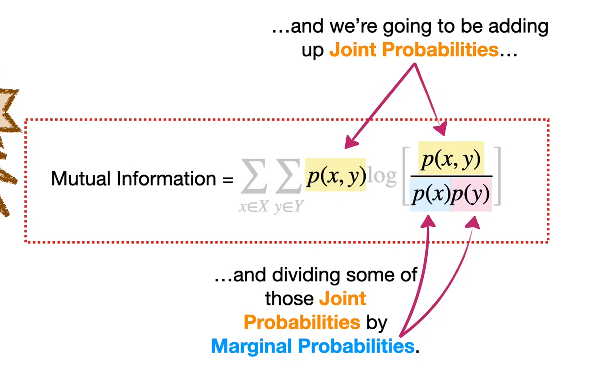
Mutual Information
The mutual information between two random variables X and Y is
I(X;Y)=H(X)−H(X∣Y)=H(Y)−H(Y∣X)I(X;Y) = H(X) - H(X|Y) = H(Y) - H(Y|X)I(X;Y)=H(X)−H(X∣Y)=H(Y)−H(Y∣X)
It can also be written as
I(X;Y)=H(X)+H(Y)−H(X,Y)I(X;Y) = H(X) + H(Y) - H(X,Y)I(X;Y)=H(X)+H(Y)−H(X,Y)
And in terms of distributions:
I(X;Y)=∑x,yp(x,y) logp(x,y)p(x)p(y)I(X;Y) = \sum_{x,y} p(x,y)\, \log \frac{p(x,y)}{p(x)p(y)}I(X;Y)=x,y∑p(x,y)logp(x)p(y)p(x,y)
Mutual Information as a measure of dependence
-
If I(X;Y)=0: the two variables are independent. Knowing one tells you nothing about the other.
-
If I(X;Y) is large: there is a strong dependency. Knowing one variable reduces a lot of uncertainty about the other.
2. How “large” relates to entropy
-
The maximum possible mutual information is limited by the entropy:
I(X;Y)≤min{H(X),H(Y)}.I(X;Y) \le \min\{H(X), H(Y)\}.I(X;Y)≤min{H(X),H(Y)}. -
This makes sense: you can’t learn more about Y from X than the total uncertainty H(Y) that Y has.
3. Intuition with examples
-
Independent coin flips:
I(X;Y)=0I(X;Y)=0I(X;Y)=0. -
Perfect correlation (e.g. Y=X):
I(X;Y)=H(X)=H(Y)I(X;Y)=H(X)=H(Y)I(X;Y)=H(X)=H(Y) -
Perfect anti-correlation (e.g. Y=not XY = \text{not }XY=not X):
I(X;Y)=H(X)I(X;Y)=H(X)I(X;Y)=H(X) as well — because knowing one still completely determines the other.
So yes, larger MI = stronger relationship between the two variables.
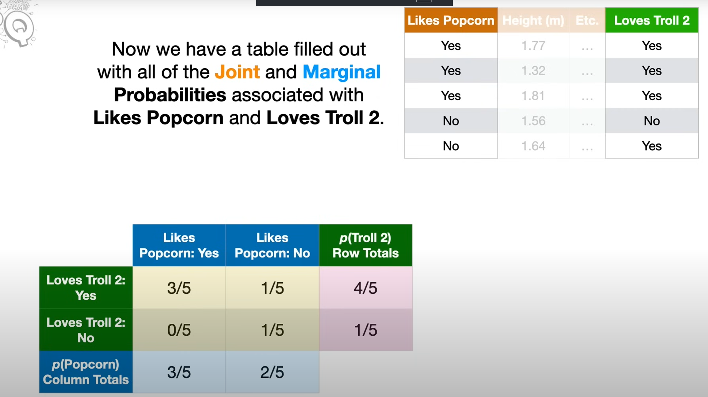
Marginal probability
- Marginal” means you’re looking at the distribution of one variable alone, ignoring the others.
- On a probability table, you literally get it by summing along the margins — that’s why it’s called marginal probability.