K近邻：从理论到实践

K近邻：从理论到实践

1. 核心思想

K近邻（KNN）是一种基于实例的监督学习方法。其基本思想是：
对于一个待分类样本，根据训练集中与其“距离”最近的 kk 个邻居的类别，通过投票或加权投票的方式决定该样本的类别。

数学表达：
设训练集为

D={(x1,y1),(x2,y2),…,(xn,yn)},xi∈Rd,yi∈{1,2,…,C}{D} = \{ (x_1,y_1), (x_2,y_2), \dots, (x_n,y_n) \}, \quad x_i \in \mathbb{R}^d, \; y_i \in \{1,2,\dots,C\}D={(x1​,y1​),(x2​,y2​),…,(xn​,yn​)},xi​∈Rd,yi​∈{1,2,…,C}

给定测试样本x，找到其最近的 kk 个邻居集合$N_k(x)$。
预测类别为：

y^(x)=arg⁡max⁡c∈{1,…,C}∑(xi,yi)∈Nk(x)1(yi=c)\hat{y}(x) = \arg\max_{c \in \{1,\dots,C\}} \sum_{(x_i,y_i) \in \mathcal{N}_k(x)} \mathbf{1}(y_i = c)y^​(x)=argc∈{1,…,C}max​(xi​,yi​)∈Nk​(x)∑​1(yi​=c)

其中，$1(\cdot )$ 是指示函数。

如果采用加权投票（考虑距离远近），则为：

y^(x)=arg⁡max⁡c∈{1,…,C}∑(xi,yi)∈Nk(x)1∥x−xi∥⋅1(yi=c)\hat{y}(x) = \arg\max_{c \in \{1,\dots,C\}} \sum_{(x_i,y_i) \in \mathcal{N}_k(x)} \frac{1}{\|x - x_i\|} \cdot \mathbf{1}(y_i = c)y^​(x)=argc∈{1,…,C}max​(xi​,yi​)∈Nk​(x)∑​∥x−xi​∥1​⋅1(yi​=c)

---

2. 距离度量

KNN 依赖距离来衡量样本相似度。常见的度量方式有：

• 欧氏距离：

$$d(x_i,x_j)=\sqrt{\sum _{l=1}^d(x_i^{(l)}-x_j^{(l)}{)}^2}$$

• 曼哈顿距离：

$$d(x_i,x_j)=\sum _{l=1}^d|x_i^{(l)}-x_j^{(l)}|$$

• 闵可夫斯基距离（推广形式）：

$$d(x_i,x_j)={\left(\sum _{l=1}^d|x_i^{(l)}-x_j^{(l)}{|}^p\right)}^{1/p}$$

---

3. k的选择与误差分析

KNN 的性能对 k 值选择敏感，体现了 近似误差 与 估计误差 的权衡。

3.1 近似误差

• 定义：模型表达能力不足，导致预测结果无法逼近真实分布。
• k 较大时：决策边界过于平滑，难以捕捉复杂模式 → 近似误差大。
• k 较小时：决策边界灵活，可以更好地拟合真实模式 → 近似误差小。

数学上，假设真实函数为 f(x)，KNN 的期望预测为：

$$\hat{f}(x)={\mathbb{E}}_{\mathcal{D}}[\hat{y}(x)]$$

则近似误差为：

$${\text{Bias}}^2(x)=({\mathbb{E}}_{\mathcal{D}}[\hat{y}(x)]-f(x){)}^2$$

3.2 估计误差

• 定义：模型对有限训练数据过于依赖，泛化性差，导致预测不稳定。
• k 较小时：极易受噪声点影响，估计误差大。
• k 较大时：结果受单个点波动影响小，估计误差小。

其数学形式为：

$$\text{Var}(x)={\mathbb{E}}_{\mathcal{D}}[(\hat{y}(x)-{\mathbb{E}}_{\mathcal{D}}[\hat{y}(x)]{)}^2]$$

3.3 总误差

$$textMSE(x)={\text{Bias}}^2(x)+\text{Var}(x)+{\sigma }^2$$

其中，${\sigma }^2$ 是不可约误差。
因此，选择合适的 k 值非常重要。

---

4. kd树的构造与搜索

由于 KNN 需要计算测试点与所有训练点的距离，时间复杂度为O(n)。为了加速，可以用 kd树进行近邻搜索。

4.1 kd树的构造

• kd树是一种对数据进行递归二分的空间划分结构。
• 每次选择一个维度（通常是方差最大的维度），按照该维度的中位数划分数据。
• 构造过程：
  1. 从根节点开始，选择一个维度作为切分轴；
  2. 找到该维度的中位数，作为节点存储值；
  3. 左子树存储小于该值的样本，右子树存储大于该值的样本；
  4. 递归进行直到样本数过少或树深度达到限制。

伪代码：

function build_kd_tree(points, depth):
if points is empty:
return None
axis = depth mod d
sort points by axis
median = len(points) // 2
node = new Node(points[median])
node.left = build_kd_tree(points[:median], depth+1)
node.right = build_kd_tree(points[median+1:], depth+1)
return node

---

4.2 kd树的搜索

kd树搜索遵循“回溯+剪枝”原则：

1. 从根节点开始，递归到叶子节点，找到测试点所属的区域；
2. 以该叶子节点为“当前最近邻”；
3. 回溯检查父节点和另一子树，若另一子树中可能存在更近邻，则递归进入；
4. 维护一个大小为 kk 的优先队列，存储当前最近的 kk 个邻居；
5. 搜索结束时队列中的点即为近邻结果。

伪代码：

function knn_search(node, target, k, depth):
if node is None:
return
axis = depth mod d
if target[axis] < node.point[axis]:
next = node.left
other = node.right
else:
next = node.right
other = node.left

function knn_search(node, target, k, depth):if node is None:returnaxis = depth mod dif target[axis] < node.point[axis]:next = node.leftother = node.rightelse:next = node.rightother = node.leftknn_search(next, target, k, depth+1)update priority queue with node.pointif |target[axis] - node.point[axis]| < current_max_distance_in_queue:knn_search(other, target, k, depth+1)

---

5. 总结

• 核心思想：KNN 通过寻找最近的 kk 个邻居来分类或回归。
• k 的选择：小 kk → 近似误差小、估计误差大（过拟合）；大 kk → 近似误差大、估计误差小（欠拟合）。
• kd树：通过空间划分加速近邻搜索，提升算法效率。

最终，KNN 的关键在于 合适的 k 值选择 和 高效的搜索结构。

---

6. K近邻用于iris数据集分类

6.1加载数据

from sklearn.datasets import load_iris
from sklearn.model_selection import train_test_splitiris = load_iris(as_frame=True)
X = iris.data[["sepal length (cm)", "sepal width (cm)"]]
y = iris.target
X_train, X_test, y_train, y_test = train_test_split(X, y, stratify=y, random_state=0)

鸢尾花数据集，as_frame=True 表示返回 pandas DataFrame 而不是 numpy 数组，方便做列选择。

这个数据集有 150 条样本，4 个特征：sepal length, sepal width, petal length, petal width。目标变量 target 有三类 (0=setosa, 1=versicolor, 2=virginica)。

6.2加载模型并可视化

import matplotlib.pyplot as plt
from sklearn.datasets import load_iris
from sklearn.model_selection import train_test_split
from sklearn.neighbors import KNeighborsClassifier
from sklearn.pipeline import Pipeline
from sklearn.preprocessing import StandardScaler
from sklearn.inspection import DecisionBoundaryDisplay
import pandas as pd
import time# 1. 载入数据
iris = load_iris(as_frame=True)
X = iris.data[["sepal length (cm)", "sepal width (cm)"]]
y = iris.target
X_train, X_test, y_train, y_test = train_test_split(X, y, stratify=y, random_state=0
)# 2. 构建 pipeline：标准化 + KNN
clf = Pipeline(steps=[("scaler", StandardScaler()),("knn", KNeighborsClassifier(n_neighbors=11))]
)# 3. 不同的 weights 和 algorithm 组合
weights_list = ["uniform", "distance"]
algorithms = ["auto", "ball_tree", "kd_tree"]# 定义结果存储表
results = []# 4. 画图：每行一个 weights，每列一个 algorithm
fig, axs = plt.subplots(nrows=len(weights_list), ncols=len(algorithms), figsize=(18, 10)
)for i, weights in enumerate(weights_list):for j, algo in enumerate(algorithms):ax = axs[i, j]# 设置参数并拟合start_train = time.time()clf.set_params(knn__weights=weights, knn__algorithm=algo).fit(X_train, y_train)end_train = time.time()start_pred = time.time()clf.predict(X_test)end_pred = time.time()acc = clf.score(X_test, y_test)results.append({"weights": weights,"algorithm": algo,"accuracy": acc,"train_time (s)": end_train - start_train,"predict_time (s)": end_pred - start_pred})# 决策边界disp = DecisionBoundaryDisplay.from_estimator(clf,X_test,response_method="predict",plot_method="pcolormesh",xlabel=iris.feature_names[0],ylabel=iris.feature_names[1],shading="auto",alpha=0.5,ax=ax,)# 训练样本点scatter = disp.ax_.scatter(X.iloc[:, 0], X.iloc[:, 1], c=y, edgecolors="k")# 图例disp.ax_.legend(scatter.legend_elements()[0],iris.target_names,loc="lower left",title="Classes",)# 子图标题ax.set_title(f"k={clf[-1].n_neighbors}, weights={weights}, algo={algo}")plt.tight_layout()
plt.show()
df_results = pd.DataFrame(results)
print(df_results)

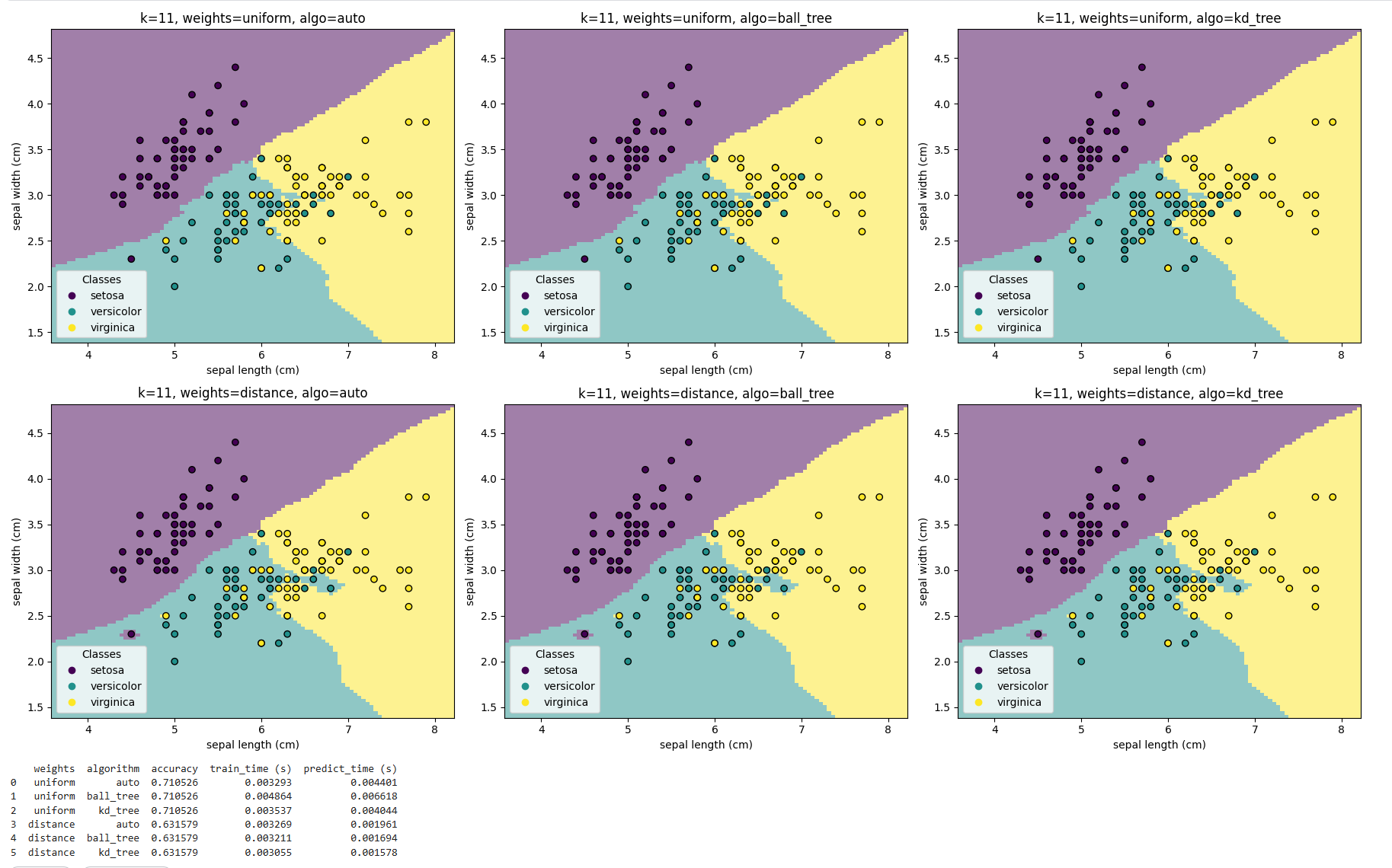
 weights  algorithm  accuracy  train_time (s)  predict_time (s)
0   uniform       auto  0.710526        0.003293          0.004401
1   uniform  ball_tree  0.710526        0.004864          0.006618
2   uniform    kd_tree  0.710526        0.003537          0.004044
3  distance       auto  0.631579        0.003269          0.001961
4  distance  ball_tree  0.631579        0.003211          0.001694
5  distance    kd_tree  0.631579        0.003055          0.001578

不同 algorithm 的表现

• auto、ball_tree、kd_tree 在相同权重下的 准确率完全一致，训练预测速度不同，这说明 搜索算法仅影响计算效率，不会改变最终分类结果。
• 这和理论一致：算法只是用不同的数据结构加速邻居查找，不会影响邻居集合本身。

不同 weights 的表现

• uniform 权重下，测试集准确率为 71.05%；
• distance 权重下，测试集准确率为 63.16%；
• 在本实验中，uniform 明显优于 distance。
• 这表明在鸢尾花数据的 前两个特征（花萼长、宽） 上，等权投票比加权投票更适合。可能原因是：
  • 特征维度少，距离加权放大了噪声点或边界点的影响；
  • 类别边界本身不完全线性，用距离权重反而削弱了多数邻居的稳定性。

结合可视化

• 从决策边界图上可以看到：

  • uniform 的边界相对平滑，更符合数据整体分布；
    eights 的表现**

• uniform 权重下，测试集准确率为 71.05%；

• distance 权重下，测试集准确率为 63.16%；

• 在本实验中，uniform 明显优于 distance。

• 这表明在鸢尾花数据的 前两个特征（花萼长、宽） 上，等权投票比加权投票更适合。可能原因是：

  • 特征维度少，距离加权放大了噪声点或边界点的影响；
  • 类别边界本身不完全线性，用距离权重反而削弱了多数邻居的稳定性。