Neural ODE原理与PyTorch实现:深度学习模型的自适应深度调节
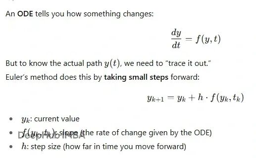
对于神经网络来说,我们已经习惯了层状网络的思维:数据进来,经过第一层,然后第二层,第三层,最后输出结果。这个过程很像流水线,每一步都是离散的。
但是现实世界的变化是连续的,比如烧开水,谁的温度不是从30度直接跳到40度,而是平滑的上生。球从山坡滚下来速度也是渐渐加快的。这些现象背后都有连续的规律在支配。
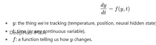
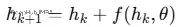
微分方程就是描述这种连续变化的语言。它不关心某个时刻的具体数值,而是告诉你"变化的速度"。比如说,温度下降得有多快?球加速得有多猛?
Neural ODE的想法很直接:自然界是连续的,神经网络要是离散的?与其让数据在固定的层之间跳跃,不如让它在时间维度上平滑地演化。
微分方程的概念
微分方程其实就是描述变化的规则。
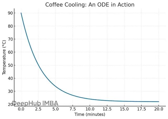
最简单的例子是咖啡冷却。刚泡好的咖啡温度高,冷却很快;温度接近室温时,冷却就变慢了。这个现象背后的规律是:冷却速度和温度差成正比。
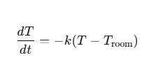
比如说:90°C的咖啡在22°C房间里,温差68度,冷却很快;30°C的咖啡在同样环境里,温差只有8度,冷却就慢得多。这就是为什么咖啡从烫嘴快速降到能喝的温度,然后就一直保持温热状态。
这不只是个咖啡的故事,它展示了动态系统的核心特征:当前状态决定了变化的方向和速度。ODE捕捉的正是这种连续演化的规律。
 # 1) 咖啡冷却曲线(指数衰减到室温)  import numpy as np
import matplotlib.pyplot as plt  # 咖啡冷却曲线 ----------
# 冷却模型参数:dT/dt = -k (T - T_room)
T0 = 90.0          # 初始温度 (°C)
T_room = 22.0      # 室温 (°C)
k = 0.35           # 冷却常数 (1/min)
t = np.linspace(0, 20, 300)  # 分钟  T = T_room + (T0 - T_room) * np.exp(-k * t)  plt.figure(figsize=(7, 5))
plt.plot(t, T, linewidth=2)
plt.title("Coffee Cooling: An ODE in Action")
plt.xlabel("Time (minutes)")
plt.ylabel("Temperature (°C)")
plt.grid(True, alpha=0.3)
coffee_path = "/data/coffee_cooling_curve.png"
plt.tight_layout()
plt.savefig(coffee_path, dpi=200, bbox_inches="tight")  plt.show()
另一个例子是球滚下山坡。球刚开始几乎不动,但重力会让它加速。滚得越快摩擦阻力越大,最终速度会趋于稳定。整个过程可以用一个ODE来描述:
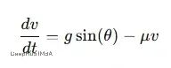
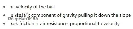
这个方程抓住了两个关键力量:重力让球加速、摩擦让球减速,速度的变化取决于这两个力的平衡。从数学上看,这个简单的方程能完整地描述球从静止到终端速度的整个过程。
 import numpy as np  import matplotlib.pyplot as plt  # ---------------- 参数 ----------------  g = 9.81           # 重力 (m/s^2)  theta_deg = 15.0   # 坡度角(度)  theta = np.deg2rad(theta_deg)  mu = 0.4           # 线性阻力系数 (1/s)  v0 = 0.0           # 初始速度 (m/s)  x0 = 0.0           # 初始位置 (m)  t_end = 12.0       # 总仿真时间 (s)  n_steps = 1200     # 积分步数  # ---------------- 时间网格 ----------------
t = np.linspace(0.0, t_end, n_steps)  # ---------------- 向量场 ----------------
def f(y, ti):  x, v = y  dv = g*np.sin(theta) - mu*v  dx = v  return np.array([dx, dv], dtype=float)  # ---------------- RK4积分器 ----------------
def rk4(f, y0, t):  y = np.zeros((len(t), len(y0)), dtype=float)  y[0] = y0  for i in range(1, len(t)):  h = t[i] - t[i-1]  ti = t[i-1]  yi = y[i-1]  k1 = f(yi, ti)  k2 = f(yi + 0.5*h*k1, ti + 0.5*h)  k3 = f(yi + 0.5*h*k2, ti + 0.5*h)  k4 = f(yi + h*k3, ti + h)  y[i] = yi + (h/6.0)*(k1 + 2*k2 + 2*k3 + k4)  return y  # ---------------- 数值积分 ----------------
y0 = np.array([x0, v0])
traj = rk4(f, y0, t)
x_num = traj[:, 0]
v_num = traj[:, 1]  # ---------------- 解析解 ----------------
v_inf = (g*np.sin(theta)) / mu if mu != 0 else np.inf
v_ana = v_inf + (v0 - v_inf) * np.exp(-mu * t)
x_ana = x0 + v_inf*t + ((v0 - v_inf)/mu) * (1.0 - np.exp(-mu*t))  # ---------------- 图1:速度 ----------------
plt.figure(figsize=(8.5, 5))
plt.plot(t, v_num, linewidth=2, label="Velocity — RK4 (numeric)")
plt.plot(t, v_ana, linewidth=2, linestyle="--", label="Velocity — analytic")
plt.axhline(v_inf, linestyle=":", label=f"Terminal velocity = {v_inf:.2f} m/s")
plt.title(f"Ball Rolling Downhill — Velocity vs Time (θ={theta_deg:.1f}°, μ={mu})")
plt.xlabel("Time (s)")
plt.ylabel("Velocity (m/s)")
plt.grid(True, alpha=0.3)
plt.legend(frameon=False)
plt.tight_layout()
vel_png = "/mnt/data/ball_downhill_velocity.png"
vel_svg = "/mnt/data/ball_downhill_velocity.svg"
plt.savefig(vel_png, dpi=220, bbox_inches="tight")
plt.savefig(vel_svg, bbox_inches="tight")
plt.show()  # ---------------- 图2:位置 ----------------
plt.figure(figsize=(8.5, 5))
plt.plot(t, x_num, linewidth=2, label="Position — RK4 (numeric)")
plt.plot(t, x_ana, linewidth=2, linestyle="--", label="Position — analytic")
plt.title(f"Ball Rolling Downhill — Position vs Time (θ={theta_deg:.1f}°, μ={mu})")
plt.xlabel("Time (s)")
plt.ylabel("Position along slope (m)")
plt.grid(True, alpha=0.3)
plt.legend(frameon=False)
plt.tight_layout()
pos_png = "/mnt/data/ball_downhill_position.png"
pos_svg = "/mnt/data/ball_downhill_position.svg"
plt.savefig(pos_png, dpi=220, bbox_inches="tight")
plt.savefig(pos_svg, bbox_inches="tight")
plt.show()  vel_png, vel_svg, pos_png, pos_svg
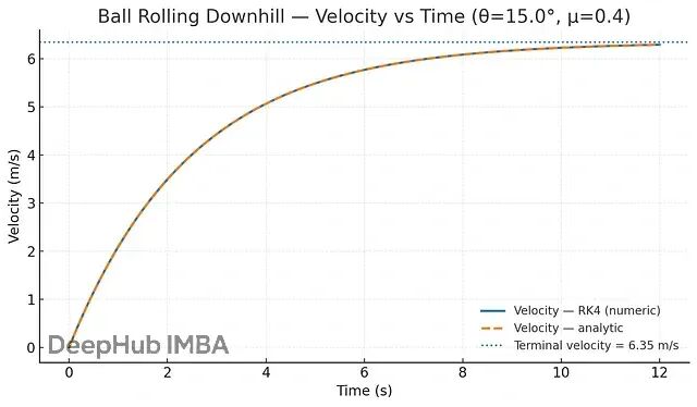
重力把球往下拉,速度快速上升,但摩擦力越来越大,最终达到终端速度。ODE完美地捕捉了这个平滑的过程。
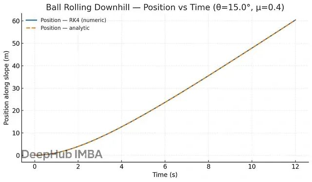
位置的变化也是如此:开始缓慢,然后加速,最后几乎匀速。这提醒我们,自然界的运动是连续的流,而不是离散的跳跃。
从深度网络到ODE
传统深度学习是离散的:
比如说ResNet的每一层都在做同样事:取当前隐藏状态,加上一些变换,然后传递给下一层。这和数值求解ODE的欧拉方法非常相似——通过小步长逼近连续变化。
或者可以说ResNet其实就是ODE的离散化版本。
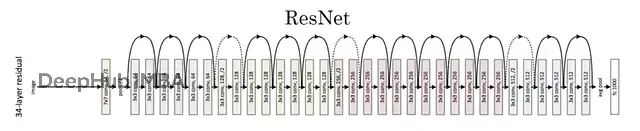
更多层应该带来更强的学习能力。但实际上网络太深反而性能下降,原因是梯度消失——学习信号在层层传递中变得越来越弱。
ResNet的关键发现是是引入残差学习。不要求每层学习完整的变换,而是学习一个"修正项":
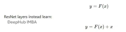
F(x)是残差,x是跳跃连接传递的原始输入。简单的说:保留原来的信息,只学习需要调整的部分。
跳跃连接字面上就是把输入x加到输出上,这让梯度能更容易地向后传播也防止了信息丢失。通过这个技巧,凯明大佬训练了152层的网络,ResNet不仅赢了2015年的ImageNet竞赛,也成为了现代计算机视觉的基础框架。
这是一个简单的ResNet块实现:
 import torch.nn as nn  # 定义单个ResNet"块"
# 每个块学习残差函数F(x),然后在最后将输入x加回
class ResNetBlock(nn.Module):  def __init__(self, in_channels, out_channels):  super().__init__()  # 第一个卷积层:  # - 应用3x3滤波器从输入中提取特征  # - padding=1确保输出大小与输入相同  self.conv1 = nn.Conv2d(in_channels, out_channels, kernel_size=3, padding=1)  # 非线性:ReLU将非线性模式引入网络  self.relu  = nn.ReLU()  # 第二个卷积层:  # - 另一个3x3滤波器来细化特征  # - 仍然保持空间大小不变  self.conv2 = nn.Conv2d(out_channels, out_channels, kernel_size=3, padding=1)  def forward(self, x):  # 将输入保存为'残差'  # 这将在稍后通过跳跃连接加回  residual = x                       # 通过第一个卷积 + ReLU激活传递输入  out = self.relu(self.conv1(x))  # 通过第二个卷积传递(还没有激活)  out = self.conv2(out)  # 将原始输入(残差)加到输出上  # 这是使ResNet特殊的"跳跃连接"  out = out + residual               # 再次应用ReLU以仅保留正激活  return self.relu(out)
关键在最后一行:返回的不是out,而是out + residual。这就是ResNet的精髓。
Neural ODE的核心思想
常规深度网络中,数据要经过固定数量的层。网络深度必须在训练前确定——10层、50层还是100层?Neural ODE彻底改变了这个思路。
不再用离散的层,而是让网络的隐藏状态在时间维度上连续演化。不是"通过100层处理输入",而是"从初始隐藏状态开始,让它按照某个规则连续演化"。
要知道隐藏状态在某个时刻的样子,就用ODE求解器,这个算法会问:状态变化有多快?需要多精确?步长应该多大?
这带来了一个关键特性:自适应深度。标准网络的深度是固定的,但Neural ODE中求解器自己决定需要多少步。简单数据用几步就够了,复杂数据就多用几步,网络在计算过程中自动调整"深度"。
Neural ODE的几个优势:
内存效率:不需要存储所有中间激活,只要起点和终点。
自适应计算:简单问题少用计算,复杂问题多用计算。
连续建模:天然适合物理、生物、金融等连续变化的系统。
可逆性:对生成模型特别有用。
构建Neural ODE
torchdiffeq
是PyTorch的Neural ODE库:
pip install torchdiffeq import torch import torch.nn as nn from torchdiffeq import odeint
定义ODE的动力学函数:
 import torch
import torch.nn as nn  class ODEFunc(nn.Module):  def __init__(self):  super().__init__()  # 定义参数化f_theta(h)的神经网络  # 输入:h(大小为2的状态向量)  # 输出:dh/dt(h的变化率,也是大小2)  self.net = nn.Sequential(  nn.Linear(2, 50),   # 层:从2D状态 -> 50个隐藏单元  nn.Tanh(),          # 非线性激活以获得灵活性  nn.Linear(50, 2)    # 层:从50个隐藏单元 -> 2D输出  )  def forward(self, t, h):  """  ODE函数的前向传播。  参数:  t : 当前时间(标量,odeint需要但这里未使用)  h : 当前状态(形状为[batch_size, 2]的张量)  返回:  dh/dt : h的估计变化率(与h形状相同)  """  return self.net(h)
这里f(h, t, θ)是个小神经网络,它描述了隐藏状态如何随时间变化。
设置初始状态和时间:
h0 = torch.tensor([[2., 0.]]) # 起始点t = torch.linspace(0, 25, 100) # 时间步长func = ODEFunc() # 你的神经ODE动力学(dh/dt = f(h))
求解ODE:
trajectory = odeint(func, h0, t) print(trajectory.shape) # (时间, 批次, 特征)
这样我们就把神经网络转换成了连续系统。
案例研究:捕食者-猎物动力学
这是个经典的生态学问题。雪兔和加拿大猞猁的种群数量呈现周期性变化:兔子多了,猞猁有足够食物,数量增加;猞猁多了,兔子被吃得多,数量下降;兔子少了,猞猁没东西吃,数量也下降;猞猁少了,兔子又开始繁盛…这个循环不断重复。
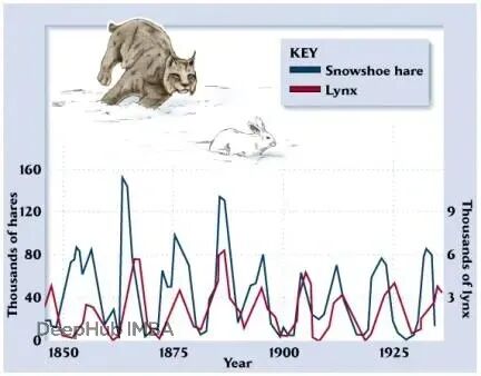
这种动力学天然适合用微分方程建模,Neural ODE可以直接从历史数据中学习这个系统的演化规律,产生平滑的轨迹,并预测未来的种群变化。
为什么捕食者-猎物系统适合用ODE建模?
连续变化:种群不会突然跳跃,而是随着动物的出生、死亡平滑变化。
相互依赖:猎物的增长率不只取决于自身繁殖,还取决于捕食者数量。捕食者的生存也依赖猎物的可获得性。
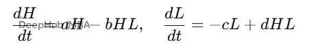
这里H是兔子,L是猞猁,a是猎物出生率,b是捕食率,c是捕食者死亡率,d是捕食者繁殖率。
反馈循环:更多猎物→捕食者增长→猎物衰落→捕食者饿死→猎物恢复→周期继续。这些反馈自然形成ODE系统。
预测能力:通过求解方程,我们不仅能描述过去的周期,还能预测或模拟不同条件下的演化。
代码实现
 !pip -q install torchdiffeq statsmodels
import math, numpy as np, torch, torch.nn as nn
import matplotlib.pyplot as plt
from torchdiffeq import odeint
from statsmodels.datasets import sunspots
DEVICE = "cuda" if torch.cuda.is_available() else "cpu"
torch.manual_seed(1337)
np.random.seed(1337)  print("Device:", DEVICE)
加载哈德逊湾公司的历史数据(1900-1920年的毛皮贸易记录):
# 真实年度毛皮计数(种群的代理),1900-1920(21年)
years = np.arange(1900, 1921, dtype=np.int32)  # 来自经典生态学教科书(四舍五入)
hares = np.array([30, 47.2, 70.2, 77.4, 36.3, 20.6, 18.1, 21.4, 22.0, 25.4,  27.1, 40.3, 57.0, 76.6, 52.3, 19.5, 11.2,  7.6, 14.6, 16.2, 24.7], dtype=np.float32)
lynx  = np.array([ 4,  6.1,  9.8, 35.2, 59.4, 41.7, 19.0, 13.0,  8.3,  9.1,  10.8, 12.6, 16.8, 20.6, 18.1,  8.0,  5.3,  3.8,  4.0,  6.5,  8.0], dtype=np.float32)  assert len(years) == len(hares) == len(lynx)
N = len(years)
print(f"Years {years[0]}–{years[-1]} (N={N})")  # 将数据放入张量并轻度标准化。
# 种群是正数且偏斜的;log1p有帮助,然后z-score用于缩放。
X_raw = np.stack([hares, lynx], axis=1)              # 形状 (N, 2)
X_log = np.log1p(X_raw)
X_mean = X_log.mean(axis=0, keepdims=True)
X_std  = X_log.std(axis=0, keepdims=True) + 1e-8
X      = (X_log - X_mean) / X_std                    # 标准化 (N, 2)  # 时间轴:居中以从0开始,使用年作为连续单位
t_year = years.astype(np.float32)
t0 = t_year[0]
t  = (t_year - t0)                                   # (N,)
t  = torch.tensor(t, dtype=torch.float32, device=DEVICE)
Y  = torch.tensor(X, dtype=torch.float32, device=DEVICE)  # (N,2)  # 训练/测试分割:拟合80%,预测最后20%
split = int(0.8 * N)
t_tr, y_tr = t[:split], Y[:split]
t_te, y_te = t[split:], Y[split:]  print("Train points:", len(t_tr), " Test points:", len(t_te))
种群数据有很大的变化范围且严格为正,所以用log1p稳定尺度,再用z-score标准化便于优化。
定义Neural ODE模型。我们直接建模2D状态[兔子,猞猁],ODE右端是个小的MLP,接收当前状态和时间特征,输出状态的变化率:
class ODEFunc(nn.Module): """ 参数化dx/dt = f_theta(x, t)。 我们包含简单的时间特征(sin/cos)以允许轻微的非平稳性。 """ def __init__(self, xdim=2, hidden=64, periods=(8.0, 11.0)): super().__init__() self.periods = torch.tensor(periods, dtype=torch.float32) # 输入:x (2) + 时间特征 (2 * [#periods](#periods)) in_dim = xdim + 2 * len(periods) self.net = nn.Sequential( nn.Linear(in_dim, hidden), nn.Tanh(), nn.Linear(hidden, hidden), nn.Tanh(), nn.Linear(hidden, xdim), ) # 温和初始化以避免早期流动爆炸 with torch.no_grad(): for m in self.net: if isinstance(m, nn.Linear): m.weight.mul_(0.1); nn.init.zeros_(m.bias) def _time_feats(self, t_scalar, batch, device): # 构建[sin(2πt/P_k), cos(2πt/P_k)]特征 tt = t_scalar * torch.ones(batch, 1, device=device) feats = [] for P in self.periods.to(device): w = 2.0 * math.pi / P feats += [torch.sin(w * tt), torch.cos(w * tt)] return torch.cat(feats, dim=1) if feats else torch.zeros(batch, 0, device=device) def forward(self, t, x): # x: (B, 2) 当前状态 B = x.shape[0] phi_t = self._time_feats(t, B, x.device) return self.net(torch.cat([x, phi_t], dim=1)) # (B,2) class NeuralODE_PredPrey(nn.Module): """ 从可学习的初始状态x0在给定时间戳上积分ODE。 我们将积分轨迹直接与观察到的x(t)比较。 """ def __init__(self, hidden=64, method="dopri5", rtol=1e-4, atol=1e-4, max_num_steps=2000): super().__init__() self.func = ODEFunc(xdim=2, hidden=hidden) # 标准化空间中的可学习初始条件 self.x0 = nn.Parameter(torch.zeros(1, 2)) # (1,2) # ODE求解器配置 self.method = method self.rtol = rtol self.atol = atol self.max_num_steps = max_num_steps def forward(self, t): """ 从x0开始在时间t上积分(广播到batch=1)。 返回轨迹(N, 1, 2) -> 我们将压缩为(N,2)。 """ opts = {"max_num_steps": self.max_num_steps} x_traj = odeint(self.func, self.x0, t, method=self.method, rtol=self.rtol, atol=self.atol, options=opts) return x_traj.squeeze(1) # (N,2)
这里加入了傅立叶时间特征(8年和11年周期)来帮助捕捉周期性行为。使用dopri5自适应求解器保持振荡特性。
训练过程中同时学习ODE动力学和初始状态,并使用早停机制避免过拟合:
# === 步骤3:训练与早停 + 最佳检查点 ===
import os, json, numpy as np, torch, torch.nn as nn
import matplotlib.pyplot as plt  # 模型(与之前相同的超参数;如果你改变了它们请调整)
model = NeuralODE_PredPrey(hidden=64, method="dopri5", rtol=1e-4, atol=1e-4).to(DEVICE)
opt    = torch.optim.AdamW(model.parameters(), lr=3e-3, weight_decay=1e-4)
loss_fn= nn.MSELoss()  # 训练配置
EPOCHS   = 3000          # 上限;如果验证停止改进我们会提前停止
PATIENCE = 50            # 等待改进的轮数(你的曲线显示~50-60最佳)
BESTPATH = "best_predprey.pt"   # 最佳模型的检查点路径  best_te = float("inf")
stale   = 0
hist    = {"epoch": [], "train_mse": [], "test_mse": []}
best_info = {"epoch": None, "test_mse": None}  for ep in range(1, EPOCHS + 1):  # ---- 在训练网格上训练 ----  model.train(); opt.zero_grad()  yhat_tr   = model(t_tr)                 # (Ntr,2)  train_mse = loss_fn(yhat_tr, y_tr)  train_mse.backward()  torch.nn.utils.clip_grad_norm_(model.parameters(), 1.0)  opt.step()  # ---- 在测试网格上验证(评估完整轨迹然后切片) ----  model.eval()  with torch.no_grad():  yhat_all = model(t)                 # (N,2)  test_mse = loss_fn(yhat_all[split:], y_te)  # ---- 日志 ----  hist["epoch"].append(ep)  hist["train_mse"].append(float(train_mse.item()))  hist["test_mse"].append(float(test_mse.item()))  # ---- 每50轮详细输出 ----  if ep % 50 == 0:  print(f"Epoch {ep:4d} | Train MSE {train_mse.item():.5f} | Test MSE {test_mse.item():.5f}")  # ---- 早停逻辑(基于测试MSE) ----  if test_mse.item() + 1e-8 < best_te:  best_te = test_mse.item()  stale   = 0  best_info["epoch"]   = ep  best_info["test_mse"]= float(best_te)  # 保存最佳检查点(仅权重)  torch.save({"model_state": model.state_dict(),  "epoch": ep,  "test_mse": float(best_te)}, BESTPATH)  else:  stale += 1  if stale >= PATIENCE:  print(f"⏹️ 在第{ep}轮早停(验证{PATIENCE}轮无改进)。"  f"最佳轮次 = {best_info['epoch']} 测试MSE = {best_info['test_mse']:.5f}")  break  # ---- 恢复最佳检查点 ----
ckpt = torch.load(BESTPATH, map_location=DEVICE)
model.load_state_dict(ckpt["model_state"])
print(f"✅ 恢复最佳模型 @ 第{ckpt['epoch']}轮 | 最佳测试MSE = {ckpt['test_mse']:.5f}")  # ---- 绘制学习曲线与最佳轮次标记 ----
epochs   = np.array(hist["epoch"], dtype=int)
train_m  = np.array(hist["train_mse"], dtype=float)
test_m   = np.array(hist["test_mse"], dtype=float)
best_ep  = int(best_info["epoch"]) if best_info["epoch"] is not None else int(epochs[np.nanargmin(test_m)])
best_val = float(best_info["test_mse"]) if best_info["test_mse"] is not None else float(np.nanmin(test_m))  plt.figure(figsize=(8,4))
plt.plot(epochs, train_m, label="Train MSE", linewidth=2)
plt.plot(epochs, test_m,  label="Test MSE",  linewidth=2, linestyle="--")
plt.axvline(best_ep, color="gray", linestyle=":", label=f"Best Test @ {best_ep} (MSE={best_val:.4f})")
plt.xlabel("Epoch"); plt.ylabel("MSE (normalized space)")
plt.title("Learning Curves (Train vs Test) with Early Stopping")
plt.grid(True, alpha=.3); plt.legend()
plt.tight_layout(); plt.show()
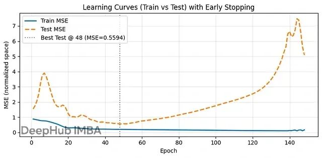
这个学习曲线展示了典型的过拟合过程。前48轮训练和测试误差一起下降,测试MSE达到最低值。之后训练误差继续改善,但测试误差开始上升——模型开始记忆训练数据的噪声,而不是学习真正的规律。这就是为什么我们需要早停机制。
可视化结果时,还需要把标准化的数据转换回原始单位,这样更容易理解:
# ===== 步骤4:评估 + 可视化 =====
import numpy as np, torch, torch.nn.functional as F
import matplotlib.pyplot as plt
from pathlib import Path
from scipy.stats import pearsonr # 1) 恢复最佳检查点(如果尚未恢复)
ckpt = torch.load(BESTPATH, map_location=DEVICE)
model.load_state_dict(ckpt["model_state"])
model.eval() # 2) 辅助函数:反标准化回原始毛皮计数
def denorm(X_norm: torch.Tensor) -> torch.Tensor: X_log = X_norm * torch.tensor(X_std.squeeze(), device=X_norm.device) + torch.tensor(X_mean.squeeze(), device=X_norm.device) return torch.expm1(X_log) # log1p的逆 # 3) 在完整时间线(训练+测试)上预测并分割
with torch.no_grad(): Yhat = model(t) # (N,2) 标准化空间
Y_den = denorm(Y) # (N,2) 原始单位
Yhat_den = denorm(Yhat) # (N,2) 原始单位 # Numpy视图
hares_obs, lynx_obs = Y_den[:,0].cpu().numpy(), Y_den[:,1].cpu().numpy()
hares_pred, lynx_pred = Yhat_den[:,0].cpu().numpy(), Yhat_den[:,1].cpu().numpy() # 4) 指标(标准化空间)
def mse(a,b): return float(np.mean((a-b)**2))
def mae(a,b): return float(np.mean(np.abs(a-b))) y_np = Y.cpu().numpy()
yhat_np = Yhat.detach().cpu().numpy()
y_tr, y_te = y_np[:split], y_np[split:]
yhat_tr, yhat_te= yhat_np[:split], yhat_np[split:] mse_tr = mse(y_tr, yhat_tr); mae_tr = mae(y_tr, yhat_tr)
mse_te = mse(y_te, yhat_te); mae_te = mae(y_te, yhat_te)
r_te = pearsonr(y_te.reshape(-1), yhat_te.reshape(-1))[0] print(f"Train MSE={mse_tr:.4f} MAE={mae_tr:.4f}")
print(f"Test MSE={mse_te:.4f} MAE={mae_te:.4f} | Pearson r (test)={r_te:.3f}") # 5) 图表
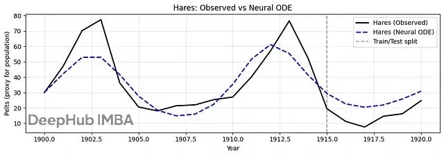
split_year = years[split-1] # (A) 时间序列叠加:兔子
plt.figure(figsize=(10,3.6))
plt.plot(years, hares_obs, 'k-', lw=2, label="Hares (Observed)")
plt.plot(years, hares_pred, 'b--', lw=2, label="Hares (Neural ODE)")
plt.axvline(split_year, color='gray', ls='--', alpha=.7, label="Train/Test split")
plt.xlabel("Year"); plt.ylabel("Pelts (proxy for population)")
plt.title("Hares: Observed vs Neural ODE")
plt.grid(alpha=.3); plt.legend(); plt.tight_layout(); plt.show() # (B) 时间序列叠加:猞猁
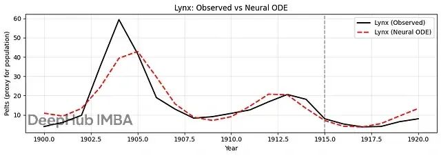
plt.figure(figsize=(10,3.6))
plt.plot(years, lynx_obs, 'k-', lw=2, label="Lynx (Observed)")
plt.plot(years, lynx_pred, 'r--', lw=2, label="Lynx (Neural ODE)")
plt.axvline(split_year, color='gray', ls='--', alpha=.7)
plt.xlabel("Year"); plt.ylabel("Pelts (proxy for population)")
plt.title("Lynx: Observed vs Neural ODE")
plt.grid(alpha=.3); plt.legend(); plt.tight_layout(); plt.show() # (C) 预测放大(仅测试区域)
plt.figure(figsize=(8,3.6))
plt.plot(years[split:], hares_obs[split:], 'k-', lw=2, label="Hares (Obs)")
plt.plot(years[split:], hares_pred[split:], 'b--', lw=2, label="Hares (Pred)")
plt.plot(years[split:], lynx_obs[split:], 'k-', lw=1.5, alpha=.6, label="Lynx (Obs)")
plt.plot(years[split:], lynx_pred[split:], 'r--', lw=1.8, label="Lynx (Pred)")
plt.xlabel("Year"); plt.ylabel("Pelts")
plt.title("Forecast Region (Test Years)")
plt.grid(alpha=.3); plt.legend(); plt.tight_layout(); plt.show() # (D) 相位肖像:兔子 vs 猞猁
plt.figure(figsize=(5.6,5.2))
plt.plot(hares_obs, lynx_obs, 'k.-', label="Observed")
plt.plot(hares_pred, lynx_pred, 'c.-', label="Neural ODE")
plt.xlabel("Hares (pelts)"); plt.ylabel("Lynx (pelts)")
plt.title("Phase Portrait: Predator–Prey Cycle")
plt.grid(alpha=.3); plt.legend(); plt.tight_layout(); plt.show() # (E) 随时间的残差(原始单位的绝对误差)
abs_err_hares = np.abs(hares_pred - hares_obs)
abs_err_lynx = np.abs(lynx_pred - lynx_obs) plt.figure(figsize=(10,3.4))
plt.plot(years, abs_err_hares, label="|Error| Hares", lw=1.8)
plt.plot(years, abs_err_lynx, label="|Error| Lynx", lw=1.8)
plt.axvline(split_year, color='gray', ls='--', alpha=.7)
plt.xlabel("Year"); plt.ylabel("Absolute Error (pelts)")
plt.title("Prediction Errors over Time")
plt.grid(alpha=.3); plt.legend(); plt.tight_layout(); plt.show() # (F) 观察 vs 预测散点图(原始单位)+ R^2
def r2_score(y_true, y_pred): y_true = np.asarray(y_true); y_pred = np.asarray(y_pred) ss_res = np.sum((y_true - y_pred)**2) ss_tot = np.sum((y_true - y_true.mean())**2) + 1e-12 return 1.0 - ss_res/ss_tot r2_hares = r2_score(hares_obs[split:], hares_pred[split:])
r2_lynx = r2_score(lynx_obs[split:], lynx_pred[split:]) plt.figure(figsize=(9,3.6))
plt.subplot(1,2,1)
plt.scatter(hares_obs[split:], hares_pred[split:], s=35, alpha=.85)
plt.plot([hares_obs.min(), hares_obs.max()], [hares_obs.min(), hares_obs.max()], 'k--', lw=1)
plt.title(f"Hares (Test): R²={r2_hares:.2f}")
plt.xlabel("Observed"); plt.ylabel("Predicted"); plt.grid(alpha=.3) plt.subplot(1,2,2)
plt.scatter(lynx_obs[split:], lynx_pred[split:], s=35, alpha=.85, color='tab:red')
plt.plot([lynx_obs.min(), lynx_obs.max()], [lynx_obs.min(), lynx_obs.max()], 'k--', lw=1)
plt.title(f"Lynx (Test): R²={r2_lynx:.2f}")
plt.xlabel("Observed"); plt.ylabel("Predicted"); plt.grid(alpha=.3) plt.tight_layout(); plt.show()
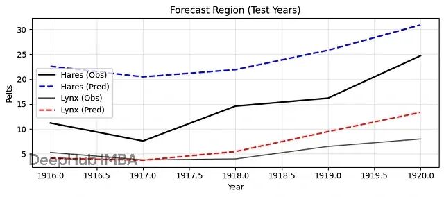
结果显示Neural ODE成功捕捉了捕食者-猎物系统的周期性动力学。模型学会了兔子和猞猁种群的相互依赖关系,能够产生平滑的预测轨迹。
如果拟合效果不够好,可以尝试:延长训练时间(
EPOCHS=5000
),增加网络容量(
hidden=96
),或者调低学习率(
lr=2e-3
)。
总结
通过一个实际案例我们看到了Neural ODE技术的强大潜力。它不仅是数学上的优雅理论,更是解决实际问题的有力工具。
Neural ODE的核心价值在于连续性思维:世界本质上是连续的,而传统深度学习的离散化可能丢失重要信息。通过引入微分方程,我们能够更自然地建模连续过程,处理不规律的时间序列数据,获得更好的数值稳定性,并实现更精确的时间建模。
当然Neural ODE也并非万能。它的计算成本较高,对初值敏感,调参也相对复杂。但随着硬件算力提升和算法优化,这些问题正在逐步解决。
正如物理学家费曼所说:"我们需要的不仅是计算能力,更是对自然规律的深刻理解。"Neural ODE正是这种理解与计算的完美结合。
https://avoid.overfit.cn/post/af8511a953524409b9f41fd27d5958b7
作者:Rayan Yassminh