当前位置：首页 > news >正文

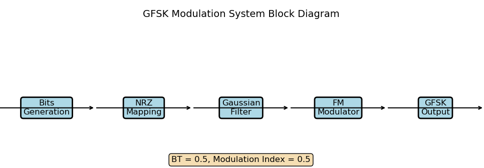
GFSK调制解调介绍(蓝牙GFSK BT=0.5)

news 2025/9/13 15:25:07

一. GFSK 概念

高斯频移键控(GFSK)是一种数字调制技术，它在FSK的基础上增加了高斯滤波处理，使频谱更加紧凑，减少带外辐射。GFSK广泛应用于蓝牙、无线传感器网络等低功耗通信系统中。

FSK：用一种载波频率来表示数字1（称为mark频率），用另一种载波频率来表示数字0（称为space频率）。例如，1用12kHz表示，0用8kHz表示。
高斯滤波： GFSK在进行FSK调制之前，先对原始的数字基带信号进行一道高斯低通滤波处理。这一步是GFSK的核心和命名来源。
目的：为什么要加这个滤波器？未经处理的数字信号是方波，其频谱很宽，边带很大。直接用它去调制频率会产生非常宽的频谱，既浪费带宽又容易干扰相邻信道。高斯滤波器可以平滑方波的跳变沿，使其没有陡峭的跳变，从而极大地压缩调制后的信号频谱，提高频谱效率。
调制指数：定义为 h = 2 * ΔF * T。其中 ΔF 是峰值频偏（载波频率最大变化量）。h=0.5 意味着 ΔF = 0.25 / T。调制指数决定了1和0对应频率之间的最小间隔。h=0.5 是最小频移键控（MSK） 的条件，能提供最佳的频谱效率和误码性能平衡。

整个流程大概如下：

优点：

高频谱效率
恒包络特性（发射机功率放大器可以工作在非线性区而不会失真，效率高）
抗干扰能力强

二. GFSK 调制流程

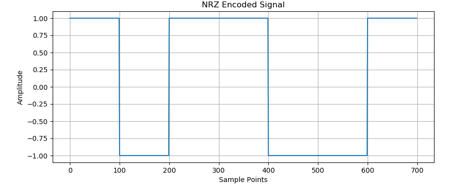
1. 生成基带NRZ信号

将输入的二进制比特流（例如 [1, 0, 1, 1, 0]）转换为非归零码（NRZ）。通常用 +1 表示比特 1，用 -1 表示比特 0。

这块比较好理解，我们直接上python代码

import numpy as np
import matplotlib.pyplot as pltdef nrz_encode(bits, samples_per_bit):"""将二进制比特流转换为NRZ信号:param bits: 二进制比特序列:param samples_per_bit: 每个比特的采样点数:return: NRZ信号"""signal = np.array([])  # 初始化一个空数组，用于存储生成的信号for bit in bits:  # 遍历输入的每一个比特# 如果比特为1，生成一个长度为samples_per_bit的全1数组（表示高电平）# 如果比特为0，生成一个长度为samples_per_bit的全-1数组（表示低电平）symbol = np.ones(samples_per_bit) if bit == 1 else -np.ones(samples_per_bit)signal = np.concatenate((signal, symbol))  # 将当前比特的信号连接到总信号中return signal  # 返回完整的NRZ信号# 示例使用
bits = [1, 0, 1, 1, 0, 0, 1]  # 定义要编码的二进制序列
samples_per_bit = 100  # 设置每个比特用100个采样点表示
nrz_signal = nrz_encode(bits, samples_per_bit)  # 调用函数生成NRZ信号# 绘制结果
plt.figure(figsize=(10, 4))  # 创建图形窗口，设置大小
plt.plot(nrz_signal)  # 绘制NRZ信号
plt.title('NRZ Encoded Signal')  # 设置标题
plt.xlabel('Sample Points')  # 设置x轴标签
plt.ylabel('Amplitude')  # 设置y轴标签
plt.grid(True)  # 显示网格
plt.show()  # 显示图形

可以看到原始的数据位[1, 0, 1, 1, 0, 0, 1]

下图就是把1变为1,0变为-1

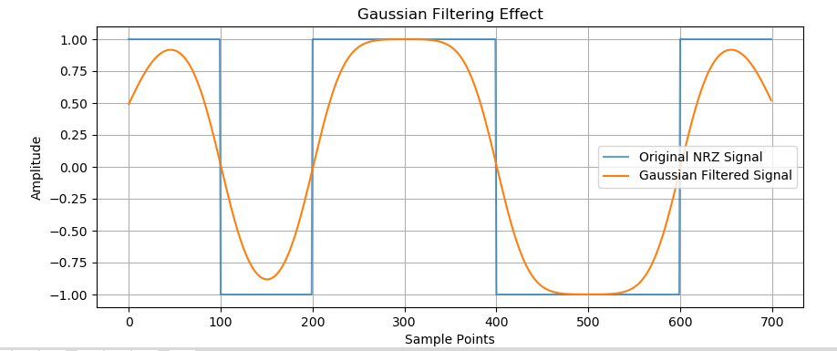
2. 高斯低通滤波

将NRZ信号通过一个截止频率由 BT 乘积决定的高斯低通滤波器。这一步将尖锐的方波脉冲平滑成类似高斯形状的脉冲。

BT乘积：这是高斯滤波器的一个关键参数。B是滤波器的3dB带宽，T是符号周期（1/比特率）。BT值越小，滤波器带宽越窄，平滑效果越强，但过多的平滑可能会导致码间串扰(ISI)。BT=0.5是一个非常经典和常用的值（例如，蓝牙技术就使用它）。

我们先来看下BT=0.5的python代码

import numpy as np
import matplotlib.pyplot as pltdef gaussian_filter(signal, bt_product, samples_per_bit):"""Apply Gaussian low-pass filter:param signal: Input signal:param bt_product: Bandwidth-time product (BT):param samples_per_bit: Number of samples per bit:return: Filtered signal"""# Calculate filter length and standard deviationfilter_length = 4 * samples_per_bit  # Filter lengthstd_dev = np.sqrt(np.log(2)) / (2 * np.pi * bt_product) * samples_per_bit# Create Gaussian filter using NumPyx = np.arange(-filter_length//2, filter_length//2)gauss_filter = np.exp(-x**2 / (2 * std_dev**2))gauss_filter = gauss_filter / np.sum(gauss_filter)  # Normalize# Apply filterfiltered_signal = np.convolve(signal, gauss_filter, mode='same')return filtered_signal# Generate NRZ signal
def nrz_encode(bits, samples_per_bit):"""Convert binary bit stream to NRZ signal:param bits: Binary bit sequence:param samples_per_bit: Number of samples per bit:return: NRZ signal"""signal = np.array([])for bit in bits:symbol = np.ones(samples_per_bit) if bit == 1 else -np.ones(samples_per_bit)signal = np.concatenate((signal, symbol))return signal# Example usage
bits = [1, 0, 1, 1, 0, 0, 1]
samples_per_bit = 100
nrz_signal = nrz_encode(bits, samples_per_bit)bt_product = 0.5  # Bandwidth-time product
filtered_signal = gaussian_filter(nrz_signal, bt_product, samples_per_bit)# Plot results
plt.figure(figsize=(10, 4))
plt.plot(nrz_signal, alpha=0.7, label='Original NRZ Signal')
plt.plot(filtered_signal, label='Gaussian Filtered Signal')
plt.title('Gaussian Filtering Effect')
plt.xlabel('Sample Points')
plt.ylabel('Amplitude')
plt.legend()
plt.grid(True)
plt.show()

我们已经在前面介绍了NRZ，我们来介绍下高斯滤波器函数

def gaussian_filter(signal, bt_product, samples_per_bit):"""Apply Gaussian low-pass filter:param signal: Input signal:param bt_product: Bandwidth-time product (BT):param samples_per_bit: Number of samples per bit:return: Filtered signal"""# Calculate filter length and standard deviationfilter_length = 4 * samples_per_bit  # Filter lengthstd_dev = np.sqrt(np.log(2)) / (2 * np.pi * bt_product) * samples_per_bit# Create Gaussian filter using NumPyx = np.arange(-filter_length//2, filter_length//2)gauss_filter = np.exp(-x**2 / (2 * std_dev**2))gauss_filter = gauss_filter / np.sum(gauss_filter)  # Normalize# Apply filterfiltered_signal = np.convolve(signal, gauss_filter, mode='same')return filtered_signal

功能解释：

参数说明：

signal：输入的NRZ信号
bt_product：带宽时间积，控制滤波器的带宽（值越小，滤波器越窄）
samples_per_bit：每个比特的采样点数

滤波器设计：

filter_length：滤波器长度设为比特长度的4倍
std_dev：计算高斯函数的标准差，基于带宽时间积和采样点数

std_dev = np.sqrt(np.log(2)) / (2 * np.pi * bt_product) * samples_per_bit

这部分对应高斯滤波器的3dB带宽与标准差的关系。对于高斯滤波器，3dB带宽 $B$ 与标准差 $\sigma$ 的关系为：

创建高斯滤波器核：使用高斯函数公式exp(-x²/(2σ²))

归一化滤波器：确保滤波后信号的总能量不变

gauss_filter = gauss_filter / np.sum(gauss_filter)

这确保了滤波器系数的总和为1，保持信号的直流分量不变，符合低通滤波器的特性。这相当于：

滤波操作：

使用np.convolve对输入信号和高斯滤波器进行卷积

filtered_signal = np.convolve(signal, gauss_filter, mode='same')

这实现了高斯滤波的数学运算：

mode='same'确保输出信号长度与输入相同

然后我们来看看不同BT值生成的波形

import numpy as np
import matplotlib.pyplot as pltdef gaussian_filter(signal, bt_product, samples_per_bit):"""Apply Gaussian low-pass filter:param signal: Input signal:param bt_product: Bandwidth-time product (BT):param samples_per_bit: Number of samples per bit:return: Filtered signal"""# Calculate filter length and standard deviationfilter_length = 4 * samples_per_bit  # Filter lengthstd_dev = np.sqrt(np.log(2)) / (2 * np.pi * bt_product) * samples_per_bit# Create Gaussian filter using NumPyx = np.arange(-filter_length//2, filter_length//2)gauss_filter = np.exp(-x**2 / (2 * std_dev**2))gauss_filter = gauss_filter / np.sum(gauss_filter)  # Normalize# Apply filterfiltered_signal = np.convolve(signal, gauss_filter, mode='same')return filtered_signal# Generate NRZ signal
def nrz_encode(bits, samples_per_bit):"""Convert binary bit stream to NRZ signal:param bits: Binary bit sequence:param samples_per_bit: Number of samples per bit:return: NRZ signal"""signal = np.array([])for bit in bits:symbol = np.ones(samples_per_bit) if bit == 1 else -np.ones(samples_per_bit)signal = np.concatenate((signal, symbol))return signal# Example usage
bits = [1, 0, 1, 1, 0, 0, 1]
samples_per_bit = 100
nrz_signal = nrz_encode(bits, samples_per_bit)# Selected BT values for comparison
bt_values = [0.2, 0.5, 0.8]
colors = ['red', 'green', 'blue']
line_styles = ['-', '--', '-.']# Create figure
plt.figure(figsize=(12, 8))# Plot original signal
plt.plot(nrz_signal, 'k-', linewidth=2, label='Original NRZ Signal')# Apply Gaussian filter with different BT values and plot
for i, bt in enumerate(bt_values):filtered_signal = gaussian_filter(nrz_signal, bt, samples_per_bit)plt.plot(filtered_signal, color=colors[i], linestyle=line_styles[i], linewidth=2, label=f'BT = {bt}')# Customize plot
plt.title('Gaussian Filtering with Different BT Values', fontsize=16)
plt.xlabel('Sample Points', fontsize=12)
plt.ylabel('Amplitude', fontsize=12)
plt.legend(loc='upper right', fontsize=10)
plt.grid(True, alpha=0.3)
plt.tight_layout()# Add annotation to explain BT effect
plt.annotate('Lower BT = More filtering (smoother)\nHigher BT = Less filtering (sharper)', xy=(0.02, 0.98), xycoords='axes fraction',fontsize=10, ha='left', va='top',bbox=dict(boxstyle='round', facecolor='wheat', alpha=0.8))# Highlight the differences at specific points
bit_transitions = [i * samples_per_bit for i in range(len(bits) + 1)]
for transition in bit_transitions:plt.axvline(x=transition, color='gray', linestyle=':', alpha=0.5)plt.show()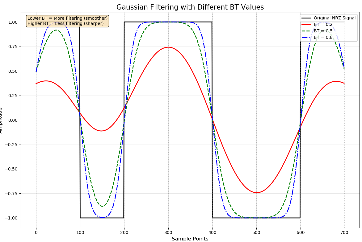

3. 频率调制

用滤波后的平滑信号去控制压控振荡器（VCO）的频率。

滤波后信号的每个采样点值 x[n] 被当作瞬时频偏。
瞬时频偏 f_dev[n] = (调制指数 * 比特率) * x[n] / 2 （因为NRZ信号的幅值是±1）。
瞬时相位 phi[n] 是瞬时频率的积分： phi[n] = 2 * pi * f_dev[n] * dt 的累积和，其中 dt 是采样间隔。

4. 生成射频信号

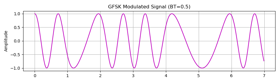
最终输出的GFSK信号是余弦（或正弦）载波，其相位由积分后的瞬时相位决定： s[n] = cos(2 * pi * fc * t[n] + phi[n])。

5. 完整gfsk代码

import numpy as np
import matplotlib.pyplot as pltdef gaussian_filter(BT, samples_per_bit, L=4):"""生成高斯滤波器BT: 带宽比特周期积samples_per_bit: 每比特采样数L: 滤波器长度（以符号周期为单位）"""# 计算滤波器参数T = 1  # 归一化符号周期B = BT / T  # 带宽alpha = np.sqrt(np.log(2)) / (2 * np.pi * B * T)  # 高斯滤波器参数# 生成时间轴t = np.arange(-L/2, L/2, 1/samples_per_bit)# 计算高斯脉冲响应h = (1 / (alpha * np.sqrt(2 * np.pi))) * np.exp(-t**2 / (2 * alpha**2))# 归一化滤波器h = h / np.sum(h)return hdef gfsk_modulate(bits, BT=0.5, samples_per_bit=100, f_dev=0.5):"""GFSK调制器bits: 输入比特序列BT: 带宽比特周期积samples_per_bit: 每比特采样数f_dev: 频率偏移（相对于符号率）"""# 将比特转换为NRZ格式 (0 -> -1, 1 -> 1)nrz_bits = np.array([1 if bit == 1 else -1 for bit in bits])# 上采样upsampled = np.zeros(len(bits) * samples_per_bit)for i, bit in enumerate(nrz_bits):upsampled[i*samples_per_bit:(i+1)*samples_per_bit] = bit# 生成高斯滤波器gaussian_taps = gaussian_filter(BT, samples_per_bit)# 应用高斯滤波器filtered = np.convolve(upsampled, gaussian_taps, mode='same')# 计算相位变化phase = np.zeros(len(filtered))for i in range(1, len(filtered)):phase[i] = phase[i-1] + 2 * np.pi * f_dev * filtered[i] / samples_per_bit# 生成GFSK信号t = np.arange(len(phase)) / samples_per_bitgfsk_signal = np.cos(2 * np.pi * t + phase)# 生成IQ信号I = np.cos(phase)Q = np.sin(phase)return gfsk_signal, phase, filtered, I, Q# 输入比特序列
bits = [1, 0, 1, 1, 0, 0, 1]# 生成GFSK信号
gfsk_signal, phase, filtered, I, Q = gfsk_modulate(bits, BT=0.5, samples_per_bit=100)# 计算频谱 - 使用NumPy的FFT
N = len(gfsk_signal)
freq = np.fft.fftfreq(N, d=1/100)  # 采样率为100Hz
spectrum = np.abs(np.fft.fftshift(np.fft.fft(gfsk_signal)))**2
spectrum_db = 10 * np.log10(spectrum / np.max(spectrum) + 1e-10)  # 转换为dB，避免log(0)# 绘制结果
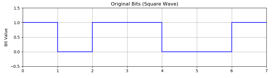
plt.figure(figsize=(14, 12))# 绘制原始比特（方波）
plt.subplot(4, 2, 1)
bit_times = np.arange(len(bits) + 1)
plt.step(bit_times, bits + [bits[-1]], 'b-', where='post')
plt.title('Original Bits (Square Wave)')
plt.ylabel('Bit Value')
plt.grid(True)
plt.ylim(-0.5, 1.5)
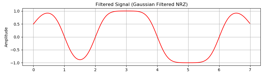
plt.xlim(0, len(bits))# 绘制滤波后的信号
plt.subplot(4, 2, 2)
t_filtered = np.arange(len(filtered)) / 100.0
plt.plot(t_filtered, filtered, 'r-')
plt.title('Filtered Signal (Gaussian Filtered NRZ)')
plt.ylabel('Amplitude')
plt.grid(True)# 绘制相位变化
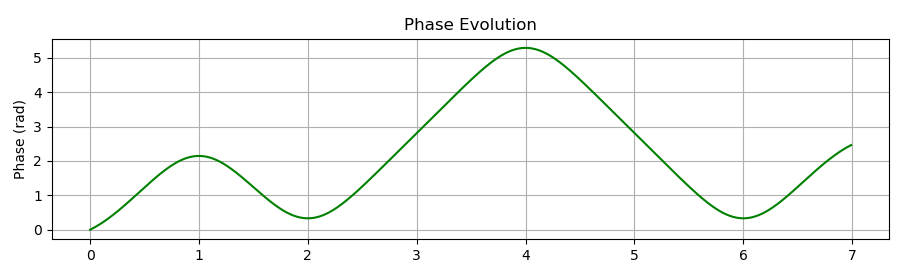
plt.subplot(4, 2, 3)
t_phase = np.arange(len(phase)) / 100.0
plt.plot(t_phase, phase, 'g-')
plt.title('Phase Evolution')
plt.ylabel('Phase (rad)')
plt.grid(True)# 绘制GFSK信号
plt.subplot(4, 2, 4)
t_signal = np.arange(len(gfsk_signal)) / 100.0
plt.plot(t_signal, gfsk_signal, 'm-')
plt.title('GFSK Modulated Signal (BT=0.5)')
plt.ylabel('Amplitude')
plt.grid(True)# 绘制IQ信号
plt.subplot(4, 2, 5)
t_iq = np.arange(len(I)) / 100.0
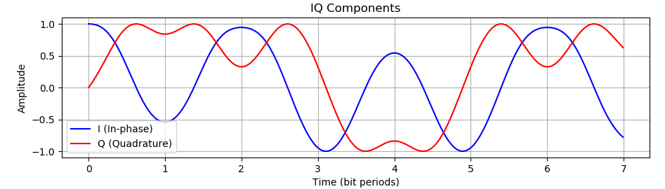
plt.plot(t_iq, I, 'b-', label='I (In-phase)')
plt.plot(t_iq, Q, 'r-', label='Q (Quadrature)')
plt.title('IQ Components')
plt.xlabel('Time (bit periods)')
plt.ylabel('Amplitude')
plt.legend()
plt.grid(True)# 绘制星座图
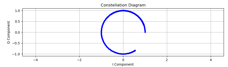
plt.subplot(4, 2, 6)
plt.plot(I, Q, 'b.')
plt.title('Constellation Diagram')
plt.xlabel('I Component')
plt.ylabel('Q Component')
plt.axis('equal')
plt.grid(True)# 绘制频谱图
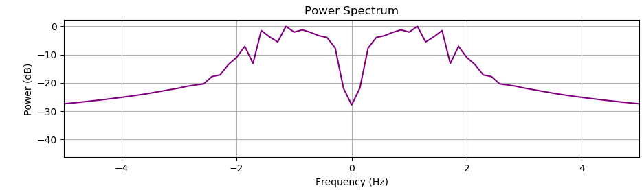
plt.subplot(4, 2, 7)
plt.plot(np.fft.fftshift(freq), spectrum_db, 'purple')
plt.title('Power Spectrum')
plt.xlabel('Frequency (Hz)')
plt.ylabel('Power (dB)')
plt.grid(True)
plt.xlim(-5, 5)  # 限制频率范围以更好地观察主瓣# 绘制时频谱图
plt.subplot(4, 2, 8)
# 使用Matplotlib的specgram函数，它不依赖SciPy
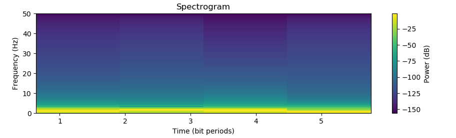
plt.specgram(gfsk_signal, Fs=100, NFFT=256, noverlap=128, cmap='viridis')
plt.title('Spectrogram')
plt.xlabel('Time (bit periods)')
plt.ylabel('Frequency (Hz)')
plt.colorbar(label='Power (dB)')plt.tight_layout()
plt.show()