吴恩达机器学习作业二:线性可分逻辑回归
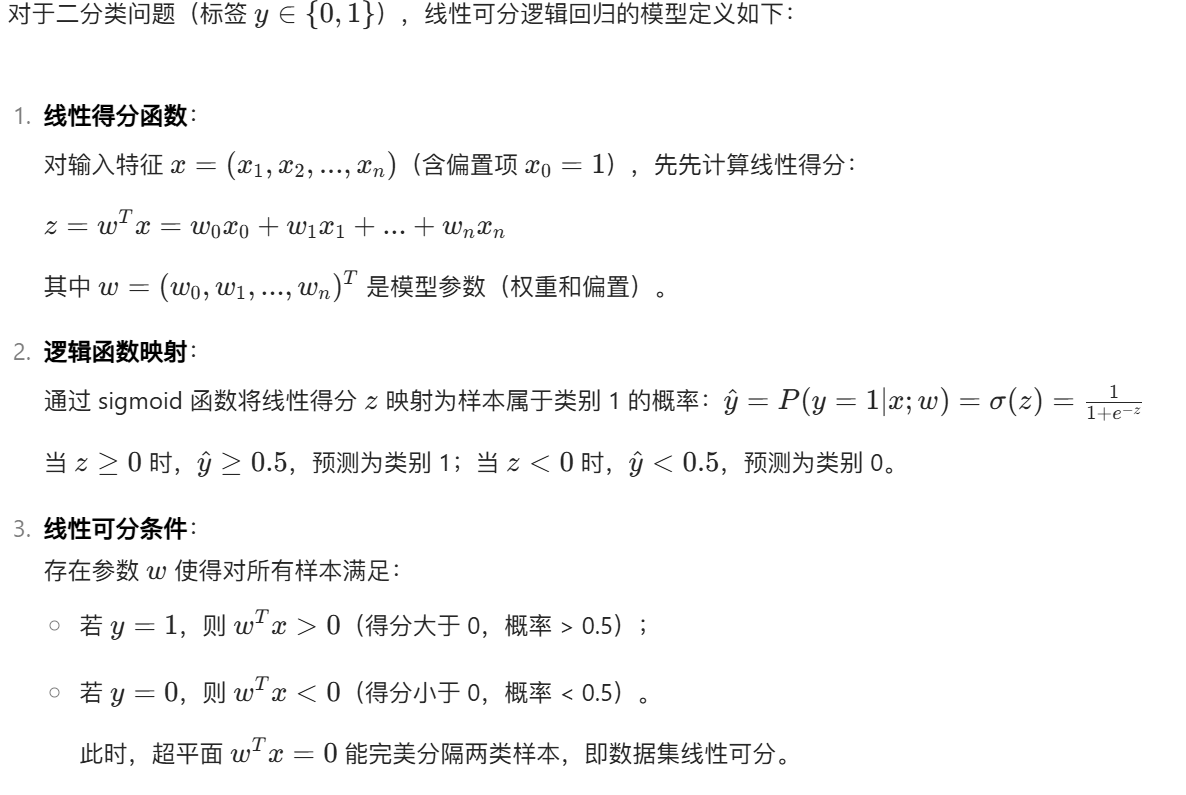
数据集在作业一
线性可分逻辑回归
线性可分逻辑回归是逻辑回归在线性可分数据集上的应用形式,它结合了线性模型的结构和逻辑回归的概率解释,用于解决二分类问题。其核心特点是:存在一个线性超平面能够将两类样本完全分开,且模型通过逻辑函数(sigmoid)将线性输出映射为类别概率。
数学定义
算法流程
1.初始化参数
2.定义损失函数
3.梯度下降
代码实现
读取数据集及可视化
import numpy as np
import pandas as pd
import matplotlib.pyplot as plt
import scipy.optimize as opt"""读取数据"""
data=pd.read_csv('ex2data1.txt',names=['Exam 1 score','Exam 2 score','Admitted'])
# print(data.head())# """数据可视化"""
# fig, ax = plt.subplots()
# ax.scatter(data[data['Admitted'] == 1]['Exam 1 score'], data[data['Admitted'] == 1]['Exam 2 score'],  c='b', marker='o', label='Admitted')
# ax.scatter(data[data['Admitted']==0]['Exam 1 score'], data[data['Admitted']==0]['Exam 2 score'], c='r', marker='x', label='Not Admitted')
# ax.legend()
# ax.set_xlabel('Exam 1 score')
# ax.set_ylabel('Exam 2 score')
# plt.show()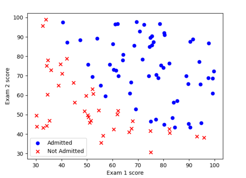
数据预处理
def getXy(data):data.insert(0,'ones',1)X=data.iloc[:,0:-1]X=X.valuesy=data.iloc[:,-1]y=y.valuesy=y.reshape((y.shape[0],1))return X,yX,y=getXy(data)损失函数(交叉熵函数)
def sigmoid(z):return 1/(1+np.exp(-z))
def cost_function(theta,X,y):m=len(y)h=sigmoid(np.dot(X,theta))J=-1/m*np.sum(y*np.log(h)+(1-y)*np.log(1-h))return Jtheta=np.zeros((3,1))
这个也是由最大似然估计推导而来。
梯度下降算法
def gradient_descent(X,y,theta,alpha,count):m=len(y)costs=[]for i in range(count):theta=theta-alpha*(1/m)*np.dot(X.T,(sigmoid(np.dot(X,theta))-y))cost=cost_function(theta,X,y)costs.append(cost)if i%1000==0:print(cost)return theta,costs预测
def predict(theta,X):prob=sigmoid(np.dot(X,theta))return [1 if x>=0.5 else 0 for x in prob]y_pred=np.array(predict(theta,X))
print(y_pred)
y_pred=y_pred.reshape((y_pred.shape[0],1))
accuracy=np.mean(y_pred==y)
print(accuracy)#准确率
可视化
fig, ax = plt.subplots()
ax.scatter(data[data['Admitted'] == 1]['Exam 1 score'], data[data['Admitted'] == 1]['Exam 2 score'],  c='b', marker='o', label='Admitted')
ax.scatter(data[data['Admitted']==0]['Exam 1 score'], data[data['Admitted']==0]['Exam 2 score'], c='r', marker='x', label='Not Admitted')
ax.legend()
ax.set_xlabel('Exam 1 score')
ax.set_ylabel('Exam 2 score')
x1=np.arange(20,100,1)
x2=(-theta[0]-theta[1]*x1)/theta[2]
ax.plot(x1,x2,c='g')
plt.show()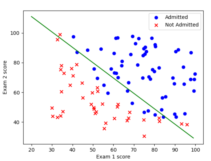
总结
读取数据集——预处理——损失函数——梯度下降算法——预测