Week 22: 深度学习补遗：Transformer+Encoder构建

Week 22: 深度学习补遗：Transformer Encoder构建

摘要

本周主要完成Transformer Encoder的代码构建，继续深挖几个主要组成部分的数学原理以及代码实现之间的细节，将理论与实践相结合。

Abstract

This week’s primary focus was on constructing the Transformer Encoder code, continuing to delve into the mathematical principles of several key components and the intricacies of their code implementation, thereby integrating theory with practice.

1. Positional Encoding 位置编码

1.1 概要

位置编码作为整个Transformer最有意思的部分之一，非常值得研究和深挖。
$$\begin{gathered} P{E}_{(pos,2i)}=\sin (\frac{pos}{10000^{\frac{2i}{d_{model}}}}) \\ P{E}_{(pos,2i+1)}=\cos (\frac{pos}{10000^{\frac{2i}{d_{model}}}}) \end{gathered}$$
Transformer的位置编码对于Token中奇偶位置的数字采取不同的位置编码。

这样设计的目的主要是由于三角函数的和差角公式的存在。
$$\{\begin{array}{rl}\sin (\alpha +\beta )& =\sin \alpha \cos \beta +\cos \alpha \sin \beta \\ \cos (\alpha +\beta )& =\cos \alpha \cos \beta -\sin \alpha \sin \beta \end{array}$$
可以得到，
$$\begin{gathered} P{E}_{(pos+k,2i)}=P{E}_{(pos,2i)}\times P{E}_{(k,2i+1)}+P{E}_{(pos,2i+1)}\times P{E}_{(k,2i)} \\ P{E}_{(pos+k,2i+1)}=P{E}_{(pos,2i+1)}\times P{E}_{(k,2i+1)}-P{E}_{(pos,2i)}\times P{E}_{(k,2i)} \end{gathered}$$
简要的说，位置编码通过三角函数的编码，利用其和差角公式的特性，对其位置信息进行加性的嵌入，同时考虑到了序列长度的因素

1.2 代码实现

class PositionalEncoding(nn.Module):def __init__(self, d_model, max_len=5000):super().__init__()pe = torch.zeros(max_len, d_model) # Initialize positional encoding matrixposition = torch.arange(0, max_len).unsqueeze(1) # [max_len, 1]div_term = torch.exp(torch.arange(0, d_model, 2) *(-math.log(10000.0) / d_model))pe[:, 0::2] = torch.sin(position * div_term) # sin for even indicespe[:, 1::2] = torch.cos(position * div_term) # cos for odd indicesself.register_buffer('pe', pe.unsqueeze(0)) # [1, max_len, d_model]def forward(self, x):return x + self.pe[:, :x.size(1)]# [:, :x.size(1)] means to get all the rows, and the first x.size(1) columns

这一份代码中有许多numpy计算中的基本技巧需要进行深挖。

比较重要的一点是计算中的溢出问题，为了避免溢出，通常使用$\log$和$e$组合替代幂运算。

div_term = torch.exp(torch.arange(0, d_model, 2) * (-math.log(10000.0) / d_model))

即
$$10000^{\frac{2i}{d_{model}}}=e^{ln(10000)\times \frac{2i}{d_{model}}}$$
通过这种变换，避免了类型溢出。

1.3 效果简析

对位置编码结果进行渲染，可以发现，10个位置均能得到不同的位置编码，又因为在计算中加入了$d_{model}$，实际上可以适用不同的序列长度。加性的将位置编码附加到Token中的各位置上，实际上就完成了位置信息的嵌入。

2. LayerNorm 层归一化

2.1 概要

层归一化是一个由Transformer推广的一项关键技术，主要是为了解决BatchNorm在时序模型中的局限性问题，其数学基础主要是将均值归一、方差归零。
$$\begin{array}{rl}\mu & \leftarrow \frac{1}{m}\sum _{i=1}^m{x}_i\\ {\sigma }^2& \leftarrow \frac{1}{m}\sum _{i=1}^m(x_i-\mu {)}^2\\ \hat{x}& \leftarrow \frac{x_i-\mu }{\sqrt{{\sigma }^2+ϵ}}\\ y& \leftarrow \gamma \hat{x}+\beta \end{array}$$
其中，$\mu$是均值，${\sigma }^2$是方差， $\gamma$和$\beta$是可学习的缩放偏移参数，$ϵ$是防止除零的小常数。

2.2 代码实现

class LayerNorm(nn.Module):def __init__(self, d_model, eps=1e-5):super().__init__()self.d_model = d_modelself.eps = epsself.gamma = nn.Parameter(torch.ones(d_model))self.beta = nn.Parameter(torch.zeros(d_model))def forward(self, x):# 计算均值和方差mean = x.mean(dim=-1, keepdim=True)var = x.var(dim=-1, keepdim=True, unbiased=False)# 归一化x_norm = (x - mean) / torch.sqrt(var + self.eps)# 缩放和偏移return self.gamma * x_norm + self.beta

3. Feed Forward Network 前馈神经网络

3.1 概要

前馈神经网络由两层线性层和一个激活函数组成，是比较基本的网络结构，但因为激活函数的存在，可以学习比较复杂的非线性特征。
$$\begin{gathered} FFN(x)=activation(x{W}_1+b_1)W_2+b_2 \\ ReLU(x)=max(0,x) \end{gathered}$$

3.2 代码实现

class FeedForward(nn.Module):def __init__(self, d_model, hidden, dropout=0.1):super().__init__()self.linear1 = nn.Linear(d_model, hidden)self.linear2 = nn.Linear(hidden, d_model)self.dropout = nn.Dropout(dropout)self.activation = nn.ReLU()def forward(self, x):x = self.linear1(x)x = self.activation(x)x = self.dropout(x)x = self.linear2(x)return x 

4. Encoder Layer构建

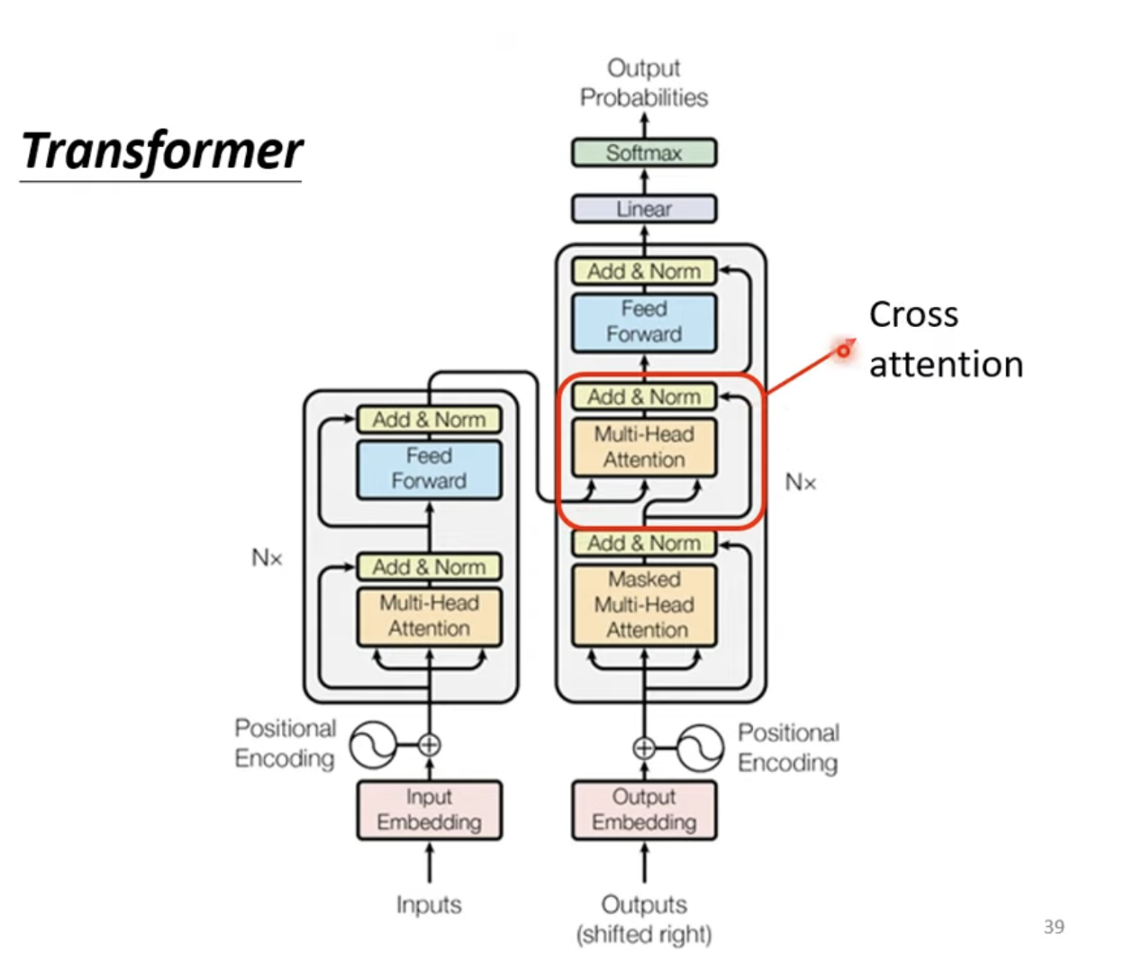
对于整个Transformer Encoder Block而言，实际上就是Input Embedding、Positional、Multi-Head Attention、FFN的组合，同时需要注意进行残差连接。

class TransformerEmbedding(nn.Module):def __init__(self, vocab_size, d_model, max_len, dropout=0.1):super().__init__()self.token_embedding = nn.Embedding(vocab_size, d_model, padding_idx=1)self.positional_encoding = PositionalEncoding(d_model, max_len)self.dropout = nn.Dropout(dropout)def forward(self, x):tok_emb = self.token_embedding(x)pos_emb = self.positional_encoding(x)return self.dropout(tok_emb + pos_emb)class EncoderLayer(nn.Module):def __init__(self, d_model, num_heads, hidden, dropout=0.1):super().__init__()self.attention = MultiHeadAttention(d_model, num_heads)self.norm1 = LayerNorm(d_model)self.dropout1 = nn.Dropout(dropout)self.ffn = FeedForward(d_model, hidden, dropout)self.norm2 = LayerNorm(d_model)self.dropout2 = nn.Dropout(dropout)def forward(self, x, mask=None):attn_output = self.attention(x, x, x, mask)x = x + self.dropout1(attn_output) # residual connectionx = self.norm1(x)ffn_output = self.ffn(x)x = x + self.dropout2(ffn_output)x = self.norm2(x)return x

这样子就完成了Transformer Encoder部分的构建。

总结

本周完成了Transformer Encoder部分的完整构建，充分的理解了包括位置编码等几项Transformer关键技术的深层数学原理以及应用效果，借助构建Transformer Encoder深入的理解Encoder乃至一个神经网络构建的基本流程以及前向传播、反向传播的数学公式在PyTorch中的实现。下周预计继续完成Decoder部分构建，继续深入理解，后续继续尝试快速利用已构建模块搭建经典论文的关键部分。