当前位置：首页 > news >正文

「日拱一码」104 MOFs + AI

news 2025/10/11 11:22:06

MOFs与AI结合

AI与MOFs的结合主要体现在以下四个层面：

1. 高性能虚拟筛选

目标：从成千上万个已知或计算机生成的虚拟MOF结构中，快速预测出对特定应用（如CO₂捕集、储氢）性能最优的少数候选材料，极大缩小实验验证的范围。
方法：
- 传统方法：使用分子模拟计算每个MOF的性能，计算成本极高，筛选数万种结构需要数百万CPU小时。
- AI方法：将MOF的结构特征（描述符）作为输入，其性能（如吸附量、选择性）作为输出，训练一个机器学习模型。一旦模型训练完成，预测一个新MOF的性能仅需毫秒级。
关键描述符：比表面积、孔体积、孔径分布、骨架密度、原子类型、几何特征等。

2. 逆向设计

目标：更高级的目标。给定一个理想的性能要求（如“在5 bar下甲烷吸附量达到200 cm³/cm³”），让AI模型生成或推荐具有这种性能的MOF化学结构（即金属和配体的组合）。
方法：使用生成式AI模型，如生成对抗网络或变分自编码器。模型学习现有MOF数据库的分布，然后在这个“化学空间”中进行探索，生成具有目标性能的新结构。

3. 合成条件预测

目标：预测合成某种MOF所需的最佳实验条件（如反应温度、时间、溶剂比例、 modulator），提高合成成功率和晶体质量。
方法：使用自然语言处理技术分析海量的科学文献，或基于实验数据库，建立从反应物和条件到合成结果（如产率、晶体尺寸）的预测模型。

4. 性质预测与分析

目标：快速预测难以通过实验直接测量或计算成本高昂的性质，如机械性能、热稳定性、催化活性等。
方法：使用深度学习模型，直接从MOF的晶体结构图（将原子视为节点，化学键视为边）学习，捕捉复杂的结构-性能关系。

代码示例

# 1. 导入必要的库
import numpy as np
import pandas as pd
import matplotlib.pyplot as plt
from sklearn.model_selection import train_test_split
from sklearn.ensemble import RandomForestRegressor
from sklearn.metrics import mean_absolute_error, r2_score
import seaborn as snsplt.rcParams['font.sans-serif'] = ['SimHei']  # 用来正常显示中文标签
plt.rcParams['axes.unicode_minus'] = False  # 用来正常显示负号
sns.set(style="whitegrid")# 2. 创建模拟的MOF数据集def create_mof_dataset(num_samples=500):np.random.seed(42)  # 设置随机种子以确保结果可重现# 生成模拟特征surface_area = np.random.normal(3000, 800, num_samples)  # 比表面积 (m²/g)pore_volume = np.random.normal(0.7, 0.2, num_samples)  # 孔体积 (cm³/g)# 确保没有负值（物理上不可能）surface_area = np.abs(surface_area)pore_volume = np.abs(pore_volume)# 根据特征生成甲烷吸附量（模拟真实的物理关系）# 吸附量大致与表面积和孔体积正相关，并加入一些非线性关系和噪声adsorption_ch4 = (0.04 * surface_area +80 * pore_volume +0.0001 * surface_area * pore_volume +  # 简单的交互项np.random.normal(0, 25, num_samples))  # 随机噪声# 创建DataFramedf = pd.DataFrame({'surface_area': surface_area,'pore_volume': pore_volume,'adsorption_ch4': adsorption_ch4})return df# 创建数据集
mof_data = create_mof_dataset(500)
print(f"数据集形状: {mof_data.shape}") # (500, 3)
print("\n数据集前5行:")
print(mof_data.head())
#    surface_area  pore_volume  adsorption_ch4
# 0   3397.371322     0.885236      241.998327
# 1   2889.388559     1.081883      225.554649
# 2   3518.150830     0.420286      175.987574
# 3   4218.423885     0.812594      217.913830
# 4   2812.677300     0.569871      175.712680# 3. 数据分析
print(f"基本统计信息:")
print(mof_data.describe())
#        surface_area  pore_volume  adsorption_ch4
# count    500.000000   500.000000      500.000000
# mean    3005.470396     0.706365      179.651283
# std      785.002598     0.195599       42.045723
# min      406.986128     0.160623       65.892806
# 25%     2439.754076     0.580942      154.556133
# 50%     3010.237717     0.705706      178.122677
# 75%     3509.426603     0.830248      205.480323
# max     6082.185193     1.226476      370.802244# 绘制特征分布
plt.figure(figsize=(15, 4))
plt.rcParams['font.sans-serif'] = ['SimHei']  # 用来正常显示中文标签
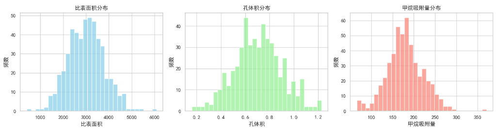
plt.rcParams['axes.unicode_minus'] = False  # 用来正常显示负号plt.subplot(1, 3, 1)
plt.hist(mof_data['surface_area'], bins=30, alpha=0.7, color='skyblue')
plt.xlabel('比表面积')
plt.ylabel('频数')
plt.title('比表面积分布')plt.subplot(1, 3, 2)
plt.hist(mof_data['pore_volume'], bins=30, alpha=0.7, color='lightgreen')
plt.xlabel('孔体积')
plt.ylabel('频数')
plt.title('孔体积分布')plt.subplot(1, 3, 3)
plt.hist(mof_data['adsorption_ch4'], bins=30, alpha=0.7, color='salmon')
plt.xlabel('甲烷吸附量')
plt.ylabel('频数')
plt.title('甲烷吸附量分布')plt.tight_layout()
plt.show()# 绘制特征与目标变量的关系
plt.figure(figsize=(12, 5))
plt.rcParams['font.sans-serif'] = ['SimHei']  # 用来正常显示中文标签
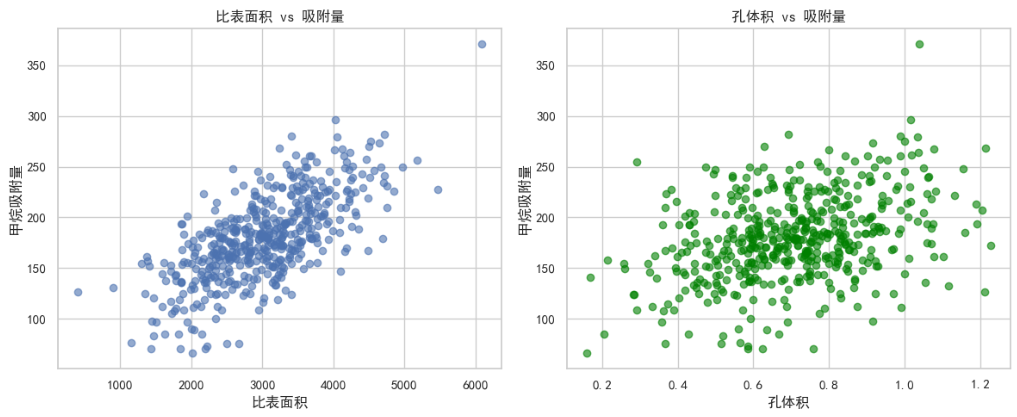
plt.rcParams['axes.unicode_minus'] = False  # 用来正常显示负号plt.subplot(1, 2, 1)
plt.scatter(mof_data['surface_area'], mof_data['adsorption_ch4'], alpha=0.6)
plt.xlabel('比表面积')
plt.ylabel('甲烷吸附量')
plt.title('比表面积 vs 吸附量')plt.subplot(1, 2, 2)
plt.scatter(mof_data['pore_volume'], mof_data['adsorption_ch4'], alpha=0.6, color='green')
plt.xlabel('孔体积')
plt.ylabel('甲烷吸附量')
plt.title('孔体积 vs 吸附量')plt.tight_layout()
plt.show()# 4. 准备机器学习数据
X = mof_data[['surface_area', 'pore_volume']]  # 特征矩阵
y = mof_data['adsorption_ch4']  # 目标变量# 将数据分为训练集和测试集
X_train, X_test, y_train, y_test = train_test_split(X, y, test_size=0.2, random_state=42
)print(f"\n--- 数据分割完成 ---")
print(f"训练集大小: {X_train.shape[0]} 个样本")  # 400
print(f"测试集大小: {X_test.shape[0]} 个样本")  # 100# 5. 创建并训练模型
print("\n--- 训练模型 ---")
model = RandomForestRegressor(n_estimators=100,  # 森林中树的数量random_state=42,  # 确保结果可重现max_depth=10  # 树的最大深度，防止过拟合
)# 训练模型
model.fit(X_train, y_train)
print("模型训练完成！")# 6. 模型评估
print("\n--- 模型评估 ---")# 在测试集上进行预测
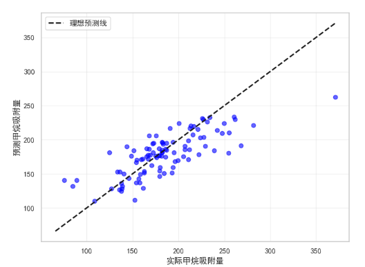
y_pred = model.predict(X_test)# 计算评估指标
mae = mean_absolute_error(y_test, y_pred)
r2 = r2_score(y_test, y_pred)print(f"平均绝对误差 (MAE): {mae:.2f} cm³/g")
print(f"决定系数 (R²): {r2:.4f}")
# 平均绝对误差 (MAE): 21.03 cm³/g
# 决定系数 (R²): 0.5717# 7. 可视化预测结果
plt.figure(figsize=(8, 6))
plt.rcParams['font.sans-serif'] = ['SimHei']  # 用来正常显示中文标签
plt.rcParams['axes.unicode_minus'] = False  # 用来正常显示负号
plt.scatter(y_test, y_pred, alpha=0.6, color='blue')
plt.plot([y.min(), y.max()], [y.min(), y.max()], 'k--', lw=2, label='理想预测线')plt.xlabel('实际甲烷吸附量')
plt.ylabel('预测甲烷吸附量')
plt.legend()
plt.grid(True, alpha=0.3)
plt.show()# 8. 特征重要性分析
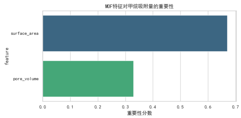
feature_importance = pd.DataFrame({'feature': X.columns,'importance': model.feature_importances_
}).sort_values('importance', ascending=False)print("\n--- 特征重要性 ---")
print("特征重要性表示每个特征对预测的贡献程度:")
for i, row in feature_importance.iterrows():print(f"{row['feature']}: {row['importance']:.4f}")# surface_area: 0.6700# pore_volume: 0.3300# 可视化特征重要性
plt.figure(figsize=(8, 4))
plt.rcParams['font.sans-serif'] = ['SimHei']  # 用来正常显示中文标签
plt.rcParams['axes.unicode_minus'] = False  # 用来正常显示负号
sns.barplot(data=feature_importance, x='importance', y='feature', palette='viridis')
plt.title('MOF特征对甲烷吸附量的重要性')
plt.xlabel('重要性分数')
plt.tight_layout()
plt.show()# 9. 使用模型进行新预测
print("\n--- 新MOF预测 ---")# 创建几个新的虚拟MOF进行预测
new_mofs = pd.DataFrame({'surface_area': [2500, 3500, 1800, 4200],  # 新MOF的比表面积'pore_volume': [0.6, 0.9, 0.4, 1.1]  # 新MOF的孔体积
})predictions = model.predict(new_mofs)
new_mofs['predicted_adsorption'] = predictionsprint("新MOF的预测结果:")
for i, row in new_mofs.iterrows():print(f"MOF {i + 1}: 表面积={row['surface_area']:.0f} m²/g, "f"孔体积={row['pore_volume']:.2f} cm³/g → "f"预测吸附量={row['predicted_adsorption']:.1f} cm³/g")
# MOF 1: 表面积=2500 m²/g, 孔体积=0.60 cm³/g → 预测吸附量=150.1 cm³/g
# MOF 2: 表面积=3500 m²/g, 孔体积=0.90 cm³/g → 预测吸附量=219.7 cm³/g
# MOF 3: 表面积=1800 m²/g, 孔体积=0.40 cm³/g → 预测吸附量=120.3 cm³/g
# MOF 4: 表面积=4200 m²/g, 孔体积=1.10 cm³/g → 预测吸附量=260.1 cm³/g