daily notes[54]

one neuron in the ANN

1. the design for neuron model of ANN was inspired by neuronbiology,the core struct include input,weight,activation function and output.
2. the output of a neuron can be simulated with the following mathmatical model.
   $$y=f\left(\sum _{i=1}^n{w}_i{x}_i+b\right)$$

• $x_i$：the i-th input from neurons in the previous level or the orignal input data.
• $w_i$：the weight corresponding to the input $x_i$ ,which means the degree of importance.
• $b$：the Bias to adjust the activiation threshold of neurons
• $f(\cdot )$：the activiation function,which enable the network to learn complex patterns through applying nonlinearity.

3. the inputted weighted summation,which is linear transformation, be firstly computed.

$$z=\sum _{i=1}^n{w}_i{x}_i+b$$
secondly,that summation will be taken to activiation function $f(z)$,through the following nonlinear function in order to similate the complicated function.

• Sigmoid：$f(z)=\frac{1}{1+e^{-z}}$,that output range from 0 to 1 ,can be apply in probability.
• ReLU：$f(z)=\max (0,z)$,can settle the matter that the vanishing gradient,to be used in the hidden level widely.
• Tanh：$f(z)=\tanh (z)$,that output range from -1 to 1,used to centralized data.
• Softmax:multi-classification output level,the output will be convert to the probability distribution.

4. to handle the batch data such as a matrix $\mathbf{X}$，the following form for computing will be apply.

$$\mathbf{y}=f(\mathbf{Xw}+\mathbf{b})$$

$\mathbf{w}$ is weighted vector ,the $\mathbf{b}$ is the bias vector.
that computation of matrix multiplication can be accelerated with GPU .
5. the entire process of a neuron’s action can be explained with the following python code using JAX.

import jax
import jax.numpy as jnp
from jax import grad, vmap, jit
import matplotlib.pyplot as plt# ------------------------------
# 1. 定义神经元模型
# ------------------------------
def neuron(params, x):"""带激活函数的单个神经元"""z = jnp.dot(x, params['w']) + params['b']  # 加权和 + 偏置return jax.nn.sigmoid(z)  # Sigmoid激活函数 (可替换为 relu/tanh)# ------------------------------
# 2. 初始化参数和超参数
# ------------------------------
input_dim = 2  # 输入特征维度
learning_rate = 0.1
epochs = 1000# 随机初始化权重和偏置
key = jax.random.PRNGKey(42)
params = {'w': jax.random.normal(key, (input_dim,)),  # 权重向量'b': 0.0  # 偏置
}# ------------------------------
# 3. 生成合成数据 (OR逻辑门)
# ------------------------------
X = jnp.array([[0, 0],[0, 1],[1, 0],[1, 1]
])
y = jnp.array([0, 1, 1, 1])  # OR逻辑门的输出# ------------------------------
# 4. 定义损失函数和梯度计算
# ------------------------------
@jit  # JIT编译加速
def loss_fn(params, X_batch, y_batch):"""均方误差损失"""predictions = vmap(neuron, in_axes=(None, 0))(params, X_batch)  # 批量预测return jnp.mean((predictions - y_batch) ** 2)compute_grads = grad(loss_fn)  # 自动微分函数# ------------------------------
# 5. 训练循环
# ------------------------------
loss_history = []for epoch in range(epochs):# 计算梯度和损失grads = compute_grads(params, X, y)loss = loss_fn(params, X, y)loss_history.append(loss)# 梯度下降更新参数params = {'w': params['w'] - learning_rate * grads['w'],'b': params['b'] - learning_rate * grads['b']}# 每100轮打印进度if epoch % 100 == 0:print(f"Epoch {epoch}, Loss: {loss:.4f}")# ------------------------------
# 6. 结果可视化
# ------------------------------
# 绘制损失曲线
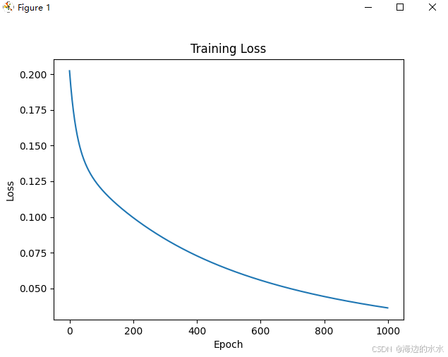
plt.plot(loss_history)
plt.xlabel("Epoch")
plt.ylabel("Loss")
plt.title("Training Loss")
plt.show()# ------------------------------
# 7. 测试预测
# ------------------------------
# 定义批量预测函数
predict = vmap(neuron, in_axes=(None, 0))# 在训练数据上测试
predictions = predict(params, X)
print("\nPredictions:")
for x, pred in zip(X, predictions):print(f"Input: {x}, Output: {pred:.4f} → Predicted class: {int(pred > 0.5)}")# ------------------------------
# 8. 输出训练后的参数
# ------------------------------
print("\nTrained parameters:")
print(f"weights: {params['w']}")
print(f"bias: {params['b']}")

conditional expectation

Monte Carlo Method is a popular method to achieve numerical calculation with randomly sampling and static simulation. it builds on law of large numbers.

import jax
import jax.numpy as jnp
from jax import randomdef exp_inverse_sample(key, lam, n_samples):u = random.uniform(key, (n_samples,))return -jnp.log(1 - u) / lamkey = random.PRNGKey(42)
samples = exp_inverse_sample(key, lam=0.5, n_samples=10_000)
print("前5个样本:", samples[:5])

import jax
import jax.numpy as jnp
from jax import random# 参数设置
lambda_Y = 0.5  # Y ~ Exp(0.5)
y_observed = 2.0  # 观测值
n_samples = 10_000# 从条件分布 X|Y ~ Exp(Y) 采样
def conditional_sample_X(key, Y):U = random.uniform(key)  # 使用单个键return -jnp.log(1 - U) / Y# 生成样本
key = random.PRNGKey(42)
keys = random.split(key, n_samples)  # 形状 (n_samples, 2)
X_samples = jax.vmap(conditional_sample_X)(keys, jnp.full((n_samples,), y_observed))# 计算条件期望
cond_expect = jnp.mean(X_samples)
print(f"E[X|Y={y_observed}] 蒙特卡洛估计: {cond_expect:.4f}")
print(f"理论值: {1/y_observed:.4f}")

binary search

1. binary search method can find the roots of equation ,which is contious function.

• let f is the function , one of the roots of f=0 must be in the range of a to b,a and b is a real number and $f(a)\ast f(b)<0$ because that f(x) will across the X-axis when x=x' and x' is in this range,x’ is a root we are seeking.
• the code can be written as follows.

import jax
import jax.numpy as jnp
from jax import jit
import jax.laxdef bisection_method(f, a, b, tol=1e-6, max_iter=100):"""使用二分法求解方程 f(x) = 0 在区间 [a, b] 内的根参数:f: 目标函数a: 区间左端点b: 区间右端点tol: 容差 (默认 1e-6)max_iter: 最大迭代次数 (默认 100)返回:近似根"""fa, fb = f(a), f(b)if fa * fb >= 0:raise ValueError("函数在区间端点必须满足 f(a)*f(b) < 0")@jitdef _bisection(a, b, fa, fb, tol, max_iter):def body_fun(val):a, b, fa, fb, _ = valc = (a + b) / 2.0fc = f(c)new_a, new_b, new_fa, new_fb = jax.lax.cond(fc * fa < 0,lambda _: (a, c, fa, fc),lambda _: (c, b, fc, fb),operand=None,)return new_a, new_b, new_fa, new_fb, fc# 使用 while_loop 替代 for 循环_, _, _, _, c = jax.lax.while_loop(lambda val: (jnp.abs(val[4]) >= tol) & (val[3] < max_iter),body_fun,(a, b, fa, fb, jnp.inf))return (a + b) / 2.0return _bisection(a, b, fa, fb, tol, max_iter)# 示例使用
if __name__ == "__main__":def f(x):return x**3 - 2*x - 5root = bisection_method(f, 1.0, 3.0)print(f"方程的近似根为: {root}")print(f"函数在根处的值: {f(root)}")

2. a new possible root will be computed as the midpoint of the two values a and b, to be verified correctness when an iteration has finished.
3. for the effect of compuational precision ,f(x) usually not equals zero and as long as the function value just is less than a very small real number.

simple iteration method

1. the simple iteration method (Fixed-point iteration method) can be used to computate the roots of equation through repeated approaching the correct root more and more closely.
2. Fixed-point iteration method intends to find a point x' which satisfies $f(x^{\prime })=x^{\prime }$.for exmaple,$f(x)=x^3+2x^2-9x+5=0$ is equivalent to $x=\frac{x^3+2x^2+5}{9}$.

• In the first place an initial root $x_1^{\prime }$ has be worked out. And in the second place, the $x_1^{\prime }$ is substituted into the function f(x) to get $f(x_1^{\prime })$ as new value $x_2^{\prime }$.until the nth attempt, the final value of $x_n^{\prime }$ is almost approximately equal to $f(x_n^{\prime })$ .
• the basic code can be as follows.

import jax
import jax.numpy as jnp
from jax import jitdef fixed_point_iteration(g, x0, tol=1e-6, max_iter=1000):"""不动点迭代法求解方程 g(x) = x参数:g: 迭代函数x0: 初始猜测值tol: 容差 (默认 1e-6)max_iter: 最大迭代次数 (默认 1000)返回:近似不动点"""def cond_fn(val):x_prev, x, i = valreturn (jnp.abs(x - x_prev) > tol) & (i < max_iter)def body_fn(val):x_prev, x, i = valreturn x, g(x), i+1# 使用 while_loop 进行迭代_, result, _ = jax.lax.while_loop(cond_fn,body_fn,(x0, g(x0), 0))return result# 使用 JIT 编译加速
fixed_point_iteration_jit = jit(fixed_point_iteration, static_argnums=(0,))# 示例使用
if __name__ == "__main__":# 定义迭代函数 (例如求解 x = cos(x))def g(x):return jnp.cos(x)# 调用不动点迭代法x_star = fixed_point_iteration_jit(g, 1.0)print(f"不动点近似值为: {x_star}")print(f"验证 g(x) - x = {g(x_star) - x_star}")

the above code ignore a different situation that the iteration is not convergent.

import jax
import jax.numpy as jnp
from jax import jit
def fixed_point_iteration_advanced(g, x0, tol=1e-6, max_iter=1000):"""带收敛诊断的不动点迭代法返回:(近似不动点, 是否收敛, 迭代次数)"""def cond_fn(val):x_prev, x, i, converged = valreturn (~converged) & (i < max_iter)def body_fn(val):x_prev, x, i, _ = valx_new = g(x)converged = jnp.abs(x_new - x) < tolreturn x, x_new, i+1, converged# 使用 while_loop 进行迭代_, result, iterations, converged = jax.lax.while_loop(cond_fn,body_fn,(x0, g(x0), 0, False))return result, converged, iterations# 使用 JIT 编译加速
fixed_point_iteration_advanced_jit = jit(fixed_point_iteration_advanced, static_argnums=(0,))# 示例使用
if __name__ == "__main__":# 定义迭代函数 (例如求解 x = e^{-x})def g(x):return jnp.exp(-x)# 调用高级版本x_star, converged, iters = fixed_point_iteration_advanced_jit(g, 0.5)print(f"不动点近似值为: {x_star}")print(f"是否收敛: {converged}")print(f"迭代次数: {iters}")

references

1. deepseek
2. 《数值计算方法》
3. 《神经网络与机器学习》