当前位置：首页 > news >正文

卷积神经网络深度解析：从基础原理到实战应用的完整指南

news 2025/9/20 7:24:30

在这里插入图片描述

🌟 Hello，我是蒋星熠Jaxonic！
🌈 在浩瀚无垠的技术宇宙中，我是一名执着的星际旅人，用代码绘制探索的轨迹。
🚀 每一个算法都是我点燃的推进器，每一行代码都是我航行的星图。
🔭 每一次性能优化都是我的天文望远镜，每一次架构设计都是我的引力弹弓。
🎻 在数字世界的协奏曲中，我既是作曲家也是首席乐手。让我们携手，在二进制星河中谱写属于极客的壮丽诗篇！

摘要

CNN不仅仅是一种算法，它更像是一把解锁视觉智能的钥匙，让机器拥有了"看见"和"理解"图像的能力。

在我的技术探索历程中，CNN始终是最令人着迷的领域之一。从最初的LeNet-5到如今的Vision Transformer，每一次架构创新都让我感受到技术进步的震撼。我记得第一次成功训练出能够识别手写数字的CNN模型时的兴奋，那种看着损失函数逐渐下降、准确率不断提升的成就感至今难忘。

CNN的核心思想源于生物视觉系统的启发，通过卷积操作、池化机制和层次化特征提取，模拟了人类视觉皮层的信息处理过程。这种设计不仅在理论上优雅，在实践中更是展现出了惊人的效果。从图像分类到目标检测，从医学影像分析到自动驾驶，CNN的应用领域之广泛令人叹为观止。

在本文中，我将带领大家深入CNN的技术内核，从数学原理到代码实现，从经典架构到最新发展，全方位解析这一改变世界的技术。我们将探讨卷积层的工作机制、池化操作的设计哲学、激活函数的选择策略，以及如何在实际项目中构建高效的CNN模型。通过丰富的代码示例和可视化图表，让每一个技术细节都变得清晰可见。

1. CNN基础原理与核心概念

1.1 卷积神经网络的生物学启发

卷积神经网络的设计灵感来源于生物视觉系统的研究。1962年，Hubel和Wiesel通过对猫视觉皮层的研究发现，视觉神经元具有局部感受野的特性，不同的神经元对特定的视觉模式（如边缘、角度）有选择性响应。

import numpy as np
import matplotlib.pyplot as plt
from scipy import ndimage# 模拟简单细胞的边缘检测功能
def simulate_simple_cell(image, orientation=0):"""模拟视觉皮层简单细胞的边缘检测功能Args:image: 输入图像orientation: 边缘方向（度）Returns:检测结果"""# 创建Gabor滤波器模拟简单细胞theta = np.radians(orientation)kernel_size = 9sigma = 2.0lambd = 4.0gamma = 0.5# 生成Gabor核x, y = np.meshgrid(np.arange(-kernel_size//2 + 1, kernel_size//2 + 1),np.arange(-kernel_size//2 + 1, kernel_size//2 + 1))x_theta = x * np.cos(theta) + y * np.sin(theta)y_theta = -x * np.sin(theta) + y * np.cos(theta)gabor = np.exp(-(x_theta**2 + gamma**2 * y_theta**2) / (2 * sigma**2)) * \np.cos(2 * np.pi * x_theta / lambd)# 应用滤波器response = ndimage.convolve(image, gabor, mode='constant')return response, gabor# 这段代码展示了如何模拟生物视觉系统中简单细胞的功能
# Gabor滤波器能够检测特定方向的边缘，这正是CNN卷积操作的生物学基础

1.2 卷积操作的数学原理

卷积操作是CNN的核心，其数学定义为：

$\int_{-\infty}^{\infty} f(\tau) g(t - \tau) d\tau$

在离散情况下，二维卷积定义为：

$\sum_m \sum_n I(m,n)K(i-m,j-n)$

import torch
import torch.nn as nn
import torch.nn.functional as Fclass ConvolutionDemo:"""卷积操作演示类"""def __init__(self):self.device = torch.device('cuda' if torch.cuda.is_available() else 'cpu')def manual_convolution(self, input_tensor, kernel, stride=1, padding=0):"""手动实现卷积操作，帮助理解卷积的计算过程Args:input_tensor: 输入张量 (batch, channels, height, width)kernel: 卷积核 (out_channels, in_channels, kernel_h, kernel_w)stride: 步长padding: 填充Returns:卷积结果"""batch_size, in_channels, in_h, in_w = input_tensor.shapeout_channels, _, kernel_h, kernel_w = kernel.shape# 计算输出尺寸out_h = (in_h + 2 * padding - kernel_h) // stride + 1out_w = (in_w + 2 * padding - kernel_w) // stride + 1# 添加填充if padding > 0:input_tensor = F.pad(input_tensor, (padding, padding, padding, padding))# 初始化输出张量output = torch.zeros(batch_size, out_channels, out_h, out_w)# 执行卷积操作for b in range(batch_size):for oc in range(out_channels):for oh in range(out_h):for ow in range(out_w):h_start = oh * strideh_end = h_start + kernel_hw_start = ow * stridew_end = w_start + kernel_w# 提取感受野receptive_field = input_tensor[b, :, h_start:h_end, w_start:w_end]# 计算卷积output[b, oc, oh, ow] = torch.sum(receptive_field * kernel[oc])return outputdef demonstrate_feature_maps(self, input_image):"""演示不同卷积核产生的特征图"""# 定义不同类型的卷积核edge_kernels = {'horizontal_edge': torch.tensor([[-1, -1, -1], [0, 0, 0], [1, 1, 1]], dtype=torch.float32),'vertical_edge': torch.tensor([[-1, 0, 1], [-1, 0, 1], [-1, 0, 1]], dtype=torch.float32),'diagonal_edge': torch.tensor([[0, 1, 0], [1, 0, -1], [0, -1, 0]], dtype=torch.float32),'blur': torch.tensor([[1, 1, 1], [1, 1, 1], [1, 1, 1]], dtype=torch.float32) / 9}feature_maps = {}for name, kernel in edge_kernels.items():# 调整kernel形状以适应conv2dkernel = kernel.unsqueeze(0).unsqueeze(0)  # (1, 1, 3, 3)feature_map = F.conv2d(input_image.unsqueeze(0).unsqueeze(0), kernel, padding=1)feature_maps[name] = feature_map.squeeze()return feature_maps# 这个类展示了卷积操作的核心机制
# 通过手动实现和特征图演示，帮助理解CNN如何提取图像特征

2. CNN架构设计与层次结构

2.1 经典CNN架构演进

图1：CNN架构演进时间线图 - 展示了从经典到现代CNN架构的发展历程

2.2 现代CNN架构实现

import torch
import torch.nn as nn
import torch.nn.functional as Fclass ResidualBlock(nn.Module):"""残差块实现 - ResNet的核心组件"""def __init__(self, in_channels, out_channels, stride=1, downsample=None):super(ResidualBlock, self).__init__()# 第一个卷积层self.conv1 = nn.Conv2d(in_channels, out_channels, kernel_size=3, stride=stride, padding=1, bias=False)self.bn1 = nn.BatchNorm2d(out_channels)# 第二个卷积层self.conv2 = nn.Conv2d(out_channels, out_channels, kernel_size=3, stride=1, padding=1, bias=False)self.bn2 = nn.BatchNorm2d(out_channels)# 下采样层（用于匹配维度）self.downsample = downsampleself.relu = nn.ReLU(inplace=True)def forward(self, x):identity = x# 第一个卷积块out = self.conv1(x)out = self.bn1(out)out = self.relu(out)# 第二个卷积块out = self.conv2(out)out = self.bn2(out)# 残差连接if self.downsample is not None:identity = self.downsample(x)out += identity  # 关键的残差连接out = self.relu(out)return outclass ModernCNN(nn.Module):"""现代CNN架构，融合多种先进技术"""def __init__(self, num_classes=1000, dropout_rate=0.5):super(ModernCNN, self).__init__()# 初始卷积层self.conv1 = nn.Conv2d(3, 64, kernel_size=7, stride=2, padding=3, bias=False)self.bn1 = nn.BatchNorm2d(64)self.relu = nn.ReLU(inplace=True)self.maxpool = nn.MaxPool2d(kernel_size=3, stride=2, padding=1)# 残差层组self.layer1 = self._make_layer(64, 64, 2, stride=1)self.layer2 = self._make_layer(64, 128, 2, stride=2)self.layer3 = self._make_layer(128, 256, 2, stride=2)self.layer4 = self._make_layer(256, 512, 2, stride=2)# 全局平均池化self.avgpool = nn.AdaptiveAvgPool2d((1, 1))# 分类器self.dropout = nn.Dropout(dropout_rate)self.fc = nn.Linear(512, num_classes)# 权重初始化self._initialize_weights()def _make_layer(self, in_channels, out_channels, blocks, stride=1):"""构建残差层组"""downsample = Noneif stride != 1 or in_channels != out_channels:downsample = nn.Sequential(nn.Conv2d(in_channels, out_channels, kernel_size=1, stride=stride, bias=False),nn.BatchNorm2d(out_channels))layers = []layers.append(ResidualBlock(in_channels, out_channels, stride, downsample))for _ in range(1, blocks):layers.append(ResidualBlock(out_channels, out_channels))return nn.Sequential(*layers)def _initialize_weights(self):"""权重初始化"""for m in self.modules():if isinstance(m, nn.Conv2d):nn.init.kaiming_normal_(m.weight, mode='fan_out', nonlinearity='relu')elif isinstance(m, nn.BatchNorm2d):nn.init.constant_(m.weight, 1)nn.init.constant_(m.bias, 0)elif isinstance(m, nn.Linear):nn.init.normal_(m.weight, 0, 0.01)nn.init.constant_(m.bias, 0)def forward(self, x):# 特征提取x = self.conv1(x)x = self.bn1(x)x = self.relu(x)x = self.maxpool(x)x = self.layer1(x)x = self.layer2(x)x = self.layer3(x)x = self.layer4(x)# 分类x = self.avgpool(x)x = torch.flatten(x, 1)x = self.dropout(x)x = self.fc(x)return x# 这个实现展示了现代CNN的核心设计原则：
# 1. 残差连接解决梯度消失问题
# 2. 批归一化加速训练
# 3. 全局平均池化减少参数
# 4. 合理的权重初始化策略

3. 卷积层与特征提取机制

3.1 多尺度特征提取

在这里插入图片描述

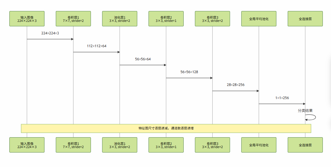
图2：CNN特征提取流程时序图 - 展示了特征图在网络中的尺寸变化过程

3.2 注意力机制增强的卷积

class ChannelAttention(nn.Module):"""通道注意力机制"""def __init__(self, in_channels, reduction=16):super(ChannelAttention, self).__init__()self.avg_pool = nn.AdaptiveAvgPool2d(1)self.max_pool = nn.AdaptiveMaxPool2d(1)# 共享的MLPself.mlp = nn.Sequential(nn.Conv2d(in_channels, in_channels // reduction, 1, bias=False),nn.ReLU(inplace=True),nn.Conv2d(in_channels // reduction, in_channels, 1, bias=False))self.sigmoid = nn.Sigmoid()def forward(self, x):# 平均池化和最大池化avg_out = self.mlp(self.avg_pool(x))max_out = self.mlp(self.max_pool(x))# 融合并生成注意力权重out = avg_out + max_outreturn self.sigmoid(out)class SpatialAttention(nn.Module):"""空间注意力机制"""def __init__(self, kernel_size=7):super(SpatialAttention, self).__init__()self.conv = nn.Conv2d(2, 1, kernel_size, padding=kernel_size//2, bias=False)self.sigmoid = nn.Sigmoid()def forward(self, x):# 通道维度的平均和最大avg_out = torch.mean(x, dim=1, keepdim=True)max_out, _ = torch.max(x, dim=1, keepdim=True)# 拼接并卷积x_cat = torch.cat([avg_out, max_out], dim=1)out = self.conv(x_cat)return self.sigmoid(out)class CBAM(nn.Module):"""卷积块注意力模块 (Convolutional Block Attention Module)"""def __init__(self, in_channels, reduction=16, kernel_size=7):super(CBAM, self).__init__()self.channel_attention = ChannelAttention(in_channels, reduction)self.spatial_attention = SpatialAttention(kernel_size)def forward(self, x):# 通道注意力x = x * self.channel_attention(x)# 空间注意力x = x * self.spatial_attention(x)return xclass AttentionConvBlock(nn.Module):"""集成注意力机制的卷积块"""def __init__(self, in_channels, out_channels, stride=1):super(AttentionConvBlock, self).__init__()self.conv1 = nn.Conv2d(in_channels, out_channels, 3, stride, 1, bias=False)self.bn1 = nn.BatchNorm2d(out_channels)self.conv2 = nn.Conv2d(out_channels, out_channels, 3, 1, 1, bias=False)self.bn2 = nn.BatchNorm2d(out_channels)# 注意力机制self.cbam = CBAM(out_channels)# 残差连接的维度匹配self.shortcut = nn.Sequential()if stride != 1 or in_channels != out_channels:self.shortcut = nn.Sequential(nn.Conv2d(in_channels, out_channels, 1, stride, bias=False),nn.BatchNorm2d(out_channels))self.relu = nn.ReLU(inplace=True)def forward(self, x):identity = self.shortcut(x)out = self.relu(self.bn1(self.conv1(x)))out = self.bn2(self.conv2(out))# 应用注意力机制out = self.cbam(out)out += identityout = self.relu(out)return out# 注意力机制让CNN能够自适应地关注重要特征
# CBAM通过通道和空间两个维度的注意力，显著提升了特征表达能力

4. 池化操作与降维策略

4.1 池化操作对比分析

池化类型	计算方式	优势	劣势	适用场景
最大池化	取窗口最大值	保留显著特征，计算简单	丢失位置信息	目标检测、分类
平均池化	取窗口平均值	保留全局信息，平滑特征	可能模糊重要特征	全局特征提取
全局平均池化	整个特征图平均	大幅减少参数，防止过拟合	丢失空间结构	分类任务最后一层
自适应池化	自适应输出尺寸	处理任意输入尺寸	计算复杂度高	多尺度输入处理
随机池化	按概率选择	增强泛化能力	训练不稳定	数据增强

4.2 高级池化策略实现

class AdvancedPooling(nn.Module):"""高级池化策略集合"""def __init__(self, in_channels, pool_type='mixed'):super(AdvancedPooling, self).__init__()self.pool_type = pool_typeif pool_type == 'mixed':# 混合池化：结合最大池化和平均池化self.max_pool = nn.MaxPool2d(2, 2)self.avg_pool = nn.AvgPool2d(2, 2)self.conv_fusion = nn.Conv2d(in_channels * 2, in_channels, 1)elif pool_type == 'stochastic':# 随机池化实现self.pool_size = 2elif pool_type == 'learnable':# 可学习池化self.pool_weights = nn.Parameter(torch.randn(1, in_channels, 2, 2))elif pool_type == 'attention':# 注意力池化self.attention_conv = nn.Conv2d(in_channels, 1, 1)self.sigmoid = nn.Sigmoid()def forward(self, x):if self.pool_type == 'mixed':max_out = self.max_pool(x)avg_out = self.avg_pool(x)mixed = torch.cat([max_out, avg_out], dim=1)return self.conv_fusion(mixed)elif self.pool_type == 'stochastic':return self.stochastic_pooling(x)elif self.pool_type == 'learnable':return F.conv2d(x, self.pool_weights, stride=2, groups=x.size(1))elif self.pool_type == 'attention':attention_map = self.sigmoid(self.attention_conv(x))return F.adaptive_avg_pool2d(x * attention_map, (x.size(2)//2, x.size(3)//2))def stochastic_pooling(self, x):"""随机池化实现"""batch_size, channels, height, width = x.size()out_h, out_w = height // self.pool_size, width // self.pool_sizeoutput = torch.zeros(batch_size, channels, out_h, out_w, device=x.device)for i in range(out_h):for j in range(out_w):h_start = i * self.pool_sizeh_end = h_start + self.pool_sizew_start = j * self.pool_sizew_end = w_start + self.pool_sizepool_region = x[:, :, h_start:h_end, w_start:w_end]if self.training:# 训练时使用随机选择pool_flat = pool_region.view(batch_size, channels, -1)probs = F.softmax(pool_flat, dim=2)indices = torch.multinomial(probs.view(-1, self.pool_size**2), 1)indices = indices.view(batch_size, channels, 1)output[:, :, i, j] = torch.gather(pool_flat, 2, indices).squeeze(2)else:# 测试时使用期望值pool_flat = pool_region.view(batch_size, channels, -1)probs = F.softmax(pool_flat, dim=2)output[:, :, i, j] = torch.sum(pool_flat * probs, dim=2)return output# 这个实现展示了多种高级池化策略
# 每种策略都有其特定的应用场景和优势

5. 激活函数与非线性变换

5.1 激活函数性能对比

在这里插入图片描述

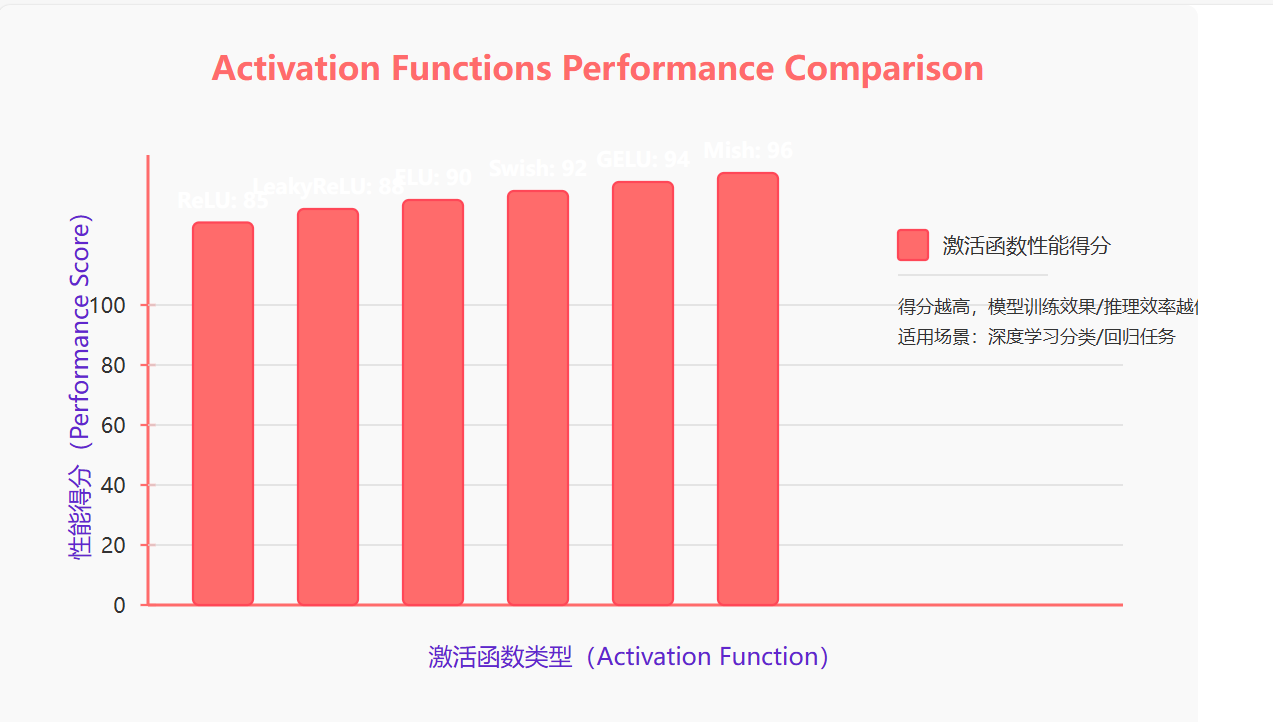
图3：激活函数性能对比图 - 展示了不同激活函数在深度网络中的表现

5.2 现代激活函数实现

import torch
import torch.nn as nn
import torch.nn.functional as F
import mathclass ModernActivations:"""现代激活函数集合"""@staticmethoddef swish(x, beta=1.0):"""Swish激活函数: x * sigmoid(β*x)"""return x * torch.sigmoid(beta * x)@staticmethoddef mish(x):"""Mish激活函数: x * tanh(softplus(x))"""return x * torch.tanh(F.softplus(x))@staticmethoddef gelu(x):"""GELU激活函数: 0.5 * x * (1 + tanh(√(2/π) * (x + 0.044715 * x³)))"""return 0.5 * x * (1 + torch.tanh(math.sqrt(2 / math.pi) * (x + 0.044715 * torch.pow(x, 3))))@staticmethoddef frelu(x, threshold=0.0):"""FReLU激活函数: max(x, threshold)，threshold可学习"""return torch.max(x, threshold)class AdaptiveActivation(nn.Module):"""自适应激活函数"""def __init__(self, num_parameters=1, init_value=0.25):super(AdaptiveActivation, self).__init__()self.num_parameters = num_parametersself.weight = nn.Parameter(torch.ones(num_parameters) * init_value)def forward(self, x):# PReLU变体：f(x) = max(0, x) + a * min(0, x)return F.relu(x) + self.weight * F.relu(-x)class ActivationComparison:"""激活函数对比实验"""def __init__(self):self.activations = {'ReLU': nn.ReLU(),'LeakyReLU': nn.LeakyReLU(0.01),'ELU': nn.ELU(),'Swish': lambda x: ModernActivations.swish(x),'Mish': lambda x: ModernActivations.mish(x),'GELU': lambda x: ModernActivations.gelu(x),'Adaptive': AdaptiveActivation()}def compare_gradients(self, x_range=(-3, 3), num_points=1000):"""比较不同激活函数的梯度特性"""x = torch.linspace(x_range[0], x_range[1], num_points, requires_grad=True)results = {}for name, activation in self.activations.items():if isinstance(activation, nn.Module):y = activation(x)else:y = activation(x)# 计算梯度grad = torch.autograd.grad(y.sum(), x, create_graph=True)[0]results[name] = {'output': y.detach(),'gradient': grad.detach(),'dead_neurons': (grad == 0).float().mean().item()}return resultsdef benchmark_performance(self, input_tensor, iterations=1000):"""性能基准测试"""results = {}for name, activation in self.activations.items():# 预热for _ in range(10):if isinstance(activation, nn.Module):_ = activation(input_tensor)else:_ = activation(input_tensor)# 计时torch.cuda.synchronize() if torch.cuda.is_available() else Nonestart_time = torch.cuda.Event(enable_timing=True) if torch.cuda.is_available() else Noneend_time = torch.cuda.Event(enable_timing=True) if torch.cuda.is_available() else Noneif torch.cuda.is_available():start_time.record()for _ in range(iterations):if isinstance(activation, nn.Module):output = activation(input_tensor)else:output = activation(input_tensor)if torch.cuda.is_available():end_time.record()torch.cuda.synchronize()elapsed_time = start_time.elapsed_time(end_time)else:elapsed_time = 0  # CPU计时需要其他方法results[name] = {'time_ms': elapsed_time,'throughput': iterations / (elapsed_time / 1000) if elapsed_time > 0 else float('inf')}return results# 这个实现提供了全面的激活函数对比框架
# 包括梯度特性分析和性能基准测试

6. 批归一化与正则化技术

6.1 正则化技术架构图

在这里插入图片描述

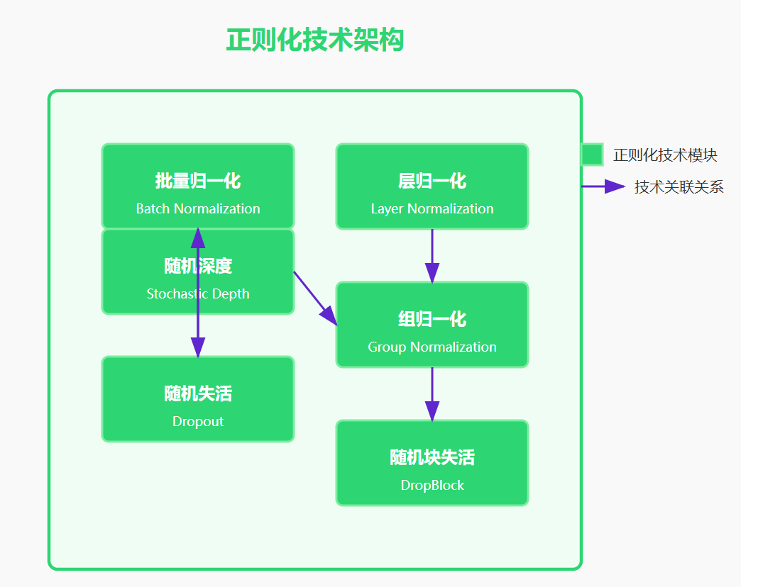
图4：正则化技术架构图 - 展示了CNN中常用的正则化方法及其关系

6.2 高级正则化技术实现

class AdvancedNormalization(nn.Module):"""高级归一化技术集合"""def __init__(self, num_features, norm_type='batch', num_groups=32, eps=1e-5, momentum=0.1):super(AdvancedNormalization, self).__init__()self.norm_type = norm_typeself.num_features = num_featuresself.eps = epsif norm_type == 'batch':self.norm = nn.BatchNorm2d(num_features, eps=eps, momentum=momentum)elif norm_type == 'layer':self.norm = nn.LayerNorm([num_features], eps=eps)elif norm_type == 'group':self.norm = nn.GroupNorm(num_groups, num_features, eps=eps)elif norm_type == 'instance':self.norm = nn.InstanceNorm2d(num_features, eps=eps)elif norm_type == 'switchable':# 可切换归一化self.batch_norm = nn.BatchNorm2d(num_features, eps=eps, momentum=momentum)self.layer_norm = nn.LayerNorm([num_features], eps=eps)self.switch_weight = nn.Parameter(torch.tensor(0.5))def forward(self, x):if self.norm_type == 'switchable':# 动态选择归一化方式batch_out = self.batch_norm(x)# Layer norm需要调整维度b, c, h, w = x.size()layer_input = x.view(b, c, -1).transpose(1, 2)  # (b, h*w, c)layer_out = self.layer_norm(layer_input)layer_out = layer_out.transpose(1, 2).view(b, c, h, w)# 加权融合return self.switch_weight * batch_out + (1 - self.switch_weight) * layer_outelse:if self.norm_type == 'layer':# Layer norm特殊处理b, c, h, w = x.size()x_reshaped = x.view(b, c, -1).transpose(1, 2)normalized = self.norm(x_reshaped)return normalized.transpose(1, 2).view(b, c, h, w)else:return self.norm(x)class DropBlock2D(nn.Module):"""DropBlock正则化 - 结构化的Dropout"""def __init__(self, drop_rate=0.1, block_size=7):super(DropBlock2D, self).__init__()self.drop_rate = drop_rateself.block_size = block_sizedef forward(self, x):if not self.training or self.drop_rate == 0:return x# 计算gamma参数gamma = self.drop_rate / (self.block_size ** 2)# 生成maskbatch_size, channels, height, width = x.size()# 采样中心点w = torch.rand(batch_size, channels, height - self.block_size + 1, width - self.block_size + 1, device=x.device)mask = (w < gamma).float()# 扩展mask到block大小mask = F.max_pool2d(mask, kernel_size=self.block_size, stride=1, padding=self.block_size // 2)# 确保mask尺寸匹配if mask.size() != x.size():mask = F.interpolate(mask, size=(height, width), mode='nearest')# 应用mask并重新缩放mask = 1 - maskreturn x * mask * mask.numel() / mask.sum()class StochasticDepth(nn.Module):"""随机深度 - 训练时随机跳过层"""def __init__(self, drop_prob=0.1):super(StochasticDepth, self).__init__()self.drop_prob = drop_probdef forward(self, x, residual):if not self.training or self.drop_prob == 0:return x + residual# 随机决定是否跳过if torch.rand(1).item() < self.drop_prob:return x  # 跳过残差连接else:return x + residualclass RegularizedConvBlock(nn.Module):"""集成多种正则化技术的卷积块"""def __init__(self, in_channels, out_channels, stride=1, norm_type='batch', drop_rate=0.1, use_dropblock=True, stochastic_depth_prob=0.1):super(RegularizedConvBlock, self).__init__()# 卷积层self.conv1 = nn.Conv2d(in_channels, out_channels, 3, stride, 1, bias=False)self.norm1 = AdvancedNormalization(out_channels, norm_type)self.conv2 = nn.Conv2d(out_channels, out_channels, 3, 1, 1, bias=False)self.norm2 = AdvancedNormalization(out_channels, norm_type)# 正则化层if use_dropblock:self.dropout = DropBlock2D(drop_rate)else:self.dropout = nn.Dropout2d(drop_rate)self.stochastic_depth = StochasticDepth(stochastic_depth_prob)# 残差连接self.shortcut = nn.Sequential()if stride != 1 or in_channels != out_channels:self.shortcut = nn.Sequential(nn.Conv2d(in_channels, out_channels, 1, stride, bias=False),AdvancedNormalization(out_channels, norm_type))self.relu = nn.ReLU(inplace=True)def forward(self, x):identity = self.shortcut(x)out = self.relu(self.norm1(self.conv1(x)))out = self.dropout(out)out = self.norm2(self.conv2(out))# 使用随机深度out = self.stochastic_depth(identity, out)out = self.relu(out)return out# 这个实现展示了现代CNN中的高级正则化技术
# 包括多种归一化方法、结构化dropout和随机深度

7. CNN训练优化策略

7.1 学习率调度策略

在这里插入图片描述

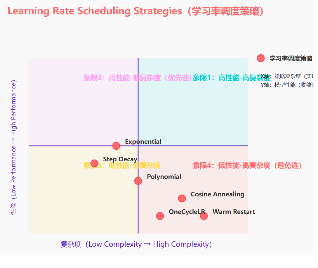
图5：学习率调度策略象限图 - 展示了不同调度策略的复杂度与性能关系

7.2 高级训练策略实现

import torch.optim as optim
from torch.optim.lr_scheduler import _LRScheduler
import mathclass WarmupCosineAnnealingLR(_LRScheduler):"""带预热的余弦退火学习率调度器"""def __init__(self, optimizer, warmup_epochs, max_epochs, eta_min=0, last_epoch=-1):self.warmup_epochs = warmup_epochsself.max_epochs = max_epochsself.eta_min = eta_minsuper(WarmupCosineAnnealingLR, self).__init__(optimizer, last_epoch)def get_lr(self):if self.last_epoch < self.warmup_epochs:# 预热阶段：线性增长return [base_lr * (self.last_epoch + 1) / self.warmup_epochs for base_lr in self.base_lrs]else:# 余弦退火阶段progress = (self.last_epoch - self.warmup_epochs) / (self.max_epochs - self.warmup_epochs)return [self.eta_min + (base_lr - self.eta_min) * (1 + math.cos(math.pi * progress)) / 2 for base_lr in self.base_lrs]class AdaptiveTrainer:"""自适应CNN训练器"""def __init__(self, model, train_loader, val_loader, device='cuda'):self.model = model.to(device)self.train_loader = train_loaderself.val_loader = val_loaderself.device = device# 优化器配置self.optimizer = self._setup_optimizer()self.scheduler = self._setup_scheduler()self.criterion = nn.CrossEntropyLoss(label_smoothing=0.1)# 训练状态self.best_acc = 0.0self.patience = 0self.max_patience = 10# 混合精度训练self.scaler = torch.cuda.amp.GradScaler() if device == 'cuda' else Nonedef _setup_optimizer(self):"""设置优化器"""# 分层学习率：不同层使用不同学习率params = []# 预训练层使用较小学习率if hasattr(self.model, 'backbone'):params.append({'params': self.model.backbone.parameters(),'lr': 1e-4,'weight_decay': 1e-4})# 新增层使用较大学习率if hasattr(self.model, 'classifier'):params.append({'params': self.model.classifier.parameters(),'lr': 1e-3,'weight_decay': 1e-4})if not params:# 默认配置params = self.model.parameters()return optim.AdamW(params, lr=1e-3, weight_decay=1e-4, betas=(0.9, 0.999))def _setup_scheduler(self):"""设置学习率调度器"""return WarmupCosineAnnealingLR(self.optimizer, warmup_epochs=5, max_epochs=100,eta_min=1e-6)def train_epoch(self):"""训练一个epoch"""self.model.train()total_loss = 0.0correct = 0total = 0for batch_idx, (data, target) in enumerate(self.train_loader):data, target = data.to(self.device), target.to(self.device)self.optimizer.zero_grad()if self.scaler is not None:# 混合精度训练with torch.cuda.amp.autocast():output = self.model(data)loss = self.criterion(output, target)self.scaler.scale(loss).backward()# 梯度裁剪self.scaler.unscale_(self.optimizer)torch.nn.utils.clip_grad_norm_(self.model.parameters(), max_norm=1.0)self.scaler.step(self.optimizer)self.scaler.update()else:# 标准训练output = self.model(data)loss = self.criterion(output, target)loss.backward()# 梯度裁剪torch.nn.utils.clip_grad_norm_(self.model.parameters(), max_norm=1.0)self.optimizer.step()# 统计total_loss += loss.item()pred = output.argmax(dim=1, keepdim=True)correct += pred.eq(target.view_as(pred)).sum().item()total += target.size(0)return total_loss / len(self.train_loader), 100. * correct / totaldef validate(self):"""验证模型"""self.model.eval()total_loss = 0.0correct = 0total = 0with torch.no_grad():for data, target in self.val_loader:data, target = data.to(self.device), target.to(self.device)if self.scaler is not None:with torch.cuda.amp.autocast():output = self.model(data)loss = self.criterion(output, target)else:output = self.model(data)loss = self.criterion(output, target)total_loss += loss.item()pred = output.argmax(dim=1, keepdim=True)correct += pred.eq(target.view_as(pred)).sum().item()total += target.size(0)acc = 100. * correct / totalreturn total_loss / len(self.val_loader), accdef train(self, epochs=100):"""完整训练流程"""for epoch in range(epochs):# 训练train_loss, train_acc = self.train_epoch()# 验证val_loss, val_acc = self.validate()# 更新学习率self.scheduler.step()# 早停检查if val_acc > self.best_acc:self.best_acc = val_accself.patience = 0# 保存最佳模型torch.save(self.model.state_dict(), 'best_model.pth')else:self.patience += 1if self.patience >= self.max_patience:print(f"Early stopping at epoch {epoch}")break# 打印进度current_lr = self.optimizer.param_groups[0]['lr']print(f'Epoch {epoch}: Train Loss: {train_loss:.4f}, Train Acc: {train_acc:.2f}%, 'f'Val Loss: {val_loss:.4f}, Val Acc: {val_acc:.2f}%, LR: {current_lr:.6f}')# 这个训练器集成了现代深度学习的最佳实践
# 包括混合精度训练、梯度裁剪、学习率预热等技术

8. CNN实际应用案例

8.1 图像分类完整实现

import torchvision.transforms as transforms
from torch.utils.data import DataLoader
import torchvision.datasets as datasetsclass ImageClassificationPipeline:"""图像分类完整流水线"""def __init__(self, num_classes=10, input_size=224):self.num_classes = num_classesself.input_size = input_sizeself.device = torch.device('cuda' if torch.cuda.is_available() else 'cpu')# 数据预处理self.train_transform = transforms.Compose([transforms.Resize((input_size, input_size)),transforms.RandomHorizontalFlip(p=0.5),transforms.RandomRotation(degrees=15),transforms.ColorJitter(brightness=0.2, contrast=0.2, saturation=0.2, hue=0.1),transforms.RandomAffine(degrees=0, translate=(0.1, 0.1), scale=(0.9, 1.1)),transforms.ToTensor(),transforms.Normalize(mean=[0.485, 0.456, 0.406], std=[0.229, 0.224, 0.225]),transforms.RandomErasing(p=0.2, scale=(0.02, 0.33), ratio=(0.3, 3.3))])self.val_transform = transforms.Compose([transforms.Resize((input_size, input_size)),transforms.ToTensor(),transforms.Normalize(mean=[0.485, 0.456, 0.406], std=[0.229, 0.224, 0.225])])# 构建模型self.model = self._build_model()def _build_model(self):"""构建分类模型"""model = ModernCNN(num_classes=self.num_classes)return model.to(self.device)def prepare_data(self, data_dir, batch_size=32, num_workers=4):"""准备数据加载器"""# 训练集train_dataset = datasets.ImageFolder(root=f'{data_dir}/train',transform=self.train_transform)# 验证集val_dataset = datasets.ImageFolder(root=f'{data_dir}/val',transform=self.val_transform)# 数据加载器train_loader = DataLoader(train_dataset, batch_size=batch_size, shuffle=True,num_workers=num_workers, pin_memory=True)val_loader = DataLoader(val_dataset, batch_size=batch_size, shuffle=False,num_workers=num_workers, pin_memory=True)return train_loader, val_loaderdef train_model(self, train_loader, val_loader, epochs=100):"""训练模型"""trainer = AdaptiveTrainer(self.model, train_loader, val_loader, self.device)trainer.train(epochs)return trainer.best_accdef evaluate_model(self, test_loader):"""评估模型性能"""self.model.eval()all_preds = []all_labels = []with torch.no_grad():for data, target in test_loader:data, target = data.to(self.device), target.to(self.device)output = self.model(data)pred = output.argmax(dim=1)all_preds.extend(pred.cpu().numpy())all_labels.extend(target.cpu().numpy())# 计算各种指标from sklearn.metrics import accuracy_score, precision_recall_fscore_support, confusion_matrixaccuracy = accuracy_score(all_labels, all_preds)precision, recall, f1, _ = precision_recall_fscore_support(all_labels, all_preds, average='weighted')cm = confusion_matrix(all_labels, all_preds)return {'accuracy': accuracy,'precision': precision,'recall': recall,'f1_score': f1,'confusion_matrix': cm}def predict_single_image(self, image_path):"""单张图像预测"""from PIL import Image# 加载和预处理图像image = Image.open(image_path).convert('RGB')input_tensor = self.val_transform(image).unsqueeze(0).to(self.device)# 预测self.model.eval()with torch.no_grad():output = self.model(input_tensor)probabilities = F.softmax(output, dim=1)predicted_class = output.argmax(dim=1).item()confidence = probabilities[0][predicted_class].item()return predicted_class, confidence, probabilities.cpu().numpy()[0]# 使用示例
if __name__ == "__main__":# 创建分类流水线pipeline = ImageClassificationPipeline(num_classes=10)# 准备数据train_loader, val_loader = pipeline.prepare_data('path/to/dataset')# 训练模型best_accuracy = pipeline.train_model(train_loader, val_loader)print(f"Best validation accuracy: {best_accuracy:.2f}%")# 评估模型metrics = pipeline.evaluate_model(val_loader)print(f"Test metrics: {metrics}")# 这个完整的实现展示了CNN在图像分类任务中的应用
# 包括数据预处理、模型训练、评估和预测的完整流程

深度学习的本质不在于模仿人脑，而在于发现数据中的模式。CNN通过层次化的特征学习，让机器拥有了超越人类的视觉感知能力。 —— Geoffrey Hinton

9. 性能优化与部署策略

9.1 模型压缩技术对比

压缩技术	压缩比	精度损失	推理速度提升	内存节省	实现复杂度
量化	2-4x	1-3%	2-3x	50-75%	中等
剪枝	2-10x	2-5%	1.5-3x	60-90%	高
知识蒸馏	3-5x	1-2%	3-5x	70-80%	中等
低秩分解	1.5-3x	0.5-2%	1.2-2x	30-60%	低
神经架构搜索	2-4x	0-1%	2-4x	50-75%	极高

9.2 模型优化实现

import torch.quantization as quantization
from torch.nn.utils import pruneclass ModelOptimizer:"""CNN模型优化器"""def __init__(self, model):self.model = modelself.original_size = self._get_model_size()def _get_model_size(self):"""计算模型大小（MB）"""param_size = 0buffer_size = 0for param in self.model.parameters():param_size += param.nelement() * param.element_size()for buffer in self.model.buffers():buffer_size += buffer.nelement() * buffer.element_size()return (param_size + buffer_size) / 1024 / 1024def quantize_model(self, calibration_loader=None):"""模型量化"""# 准备量化self.model.eval()# 动态量化（推理时量化）quantized_model = quantization.quantize_dynamic(self.model, {nn.Conv2d, nn.Linear}, dtype=torch.qint8)# 如果有校准数据，使用静态量化if calibration_loader is not None:# 设置量化配置self.model.qconfig = quantization.get_default_qconfig('fbgemm')# 准备量化quantization.prepare(self.model, inplace=True)# 校准with torch.no_grad():for data, _ in calibration_loader:self.model(data)# 转换为量化模型quantized_model = quantization.convert(self.model, inplace=False)return quantized_modeldef prune_model(self, pruning_ratio=0.3):"""模型剪枝"""# 结构化剪枝：移除整个通道for name, module in self.model.named_modules():if isinstance(module, nn.Conv2d):# L1非结构化剪枝prune.l1_unstructured(module, name='weight', amount=pruning_ratio)# 移除剪枝mask，永久删除权重prune.remove(module, 'weight')return self.modeldef knowledge_distillation(self, teacher_model, student_model, train_loader, temperature=4.0, alpha=0.7, epochs=50):"""知识蒸馏"""teacher_model.eval()student_model.train()optimizer = optim.Adam(student_model.parameters(), lr=1e-3)criterion_ce = nn.CrossEntropyLoss()criterion_kd = nn.KLDivLoss(reduction='batchmean')for epoch in range(epochs):total_loss = 0.0for data, target in train_loader:optimizer.zero_grad()# 学生模型输出student_output = student_model(data)# 教师模型输出（不计算梯度）with torch.no_grad():teacher_output = teacher_model(data)# 计算损失# 1. 标准交叉熵损失ce_loss = criterion_ce(student_output, target)# 2. 知识蒸馏损失student_soft = F.log_softmax(student_output / temperature, dim=1)teacher_soft = F.softmax(teacher_output / temperature, dim=1)kd_loss = criterion_kd(student_soft, teacher_soft) * (temperature ** 2)# 3. 总损失loss = alpha * kd_loss + (1 - alpha) * ce_lossloss.backward()optimizer.step()total_loss += loss.item()print(f'Epoch {epoch}: Loss = {total_loss / len(train_loader):.4f}')return student_modeldef optimize_for_inference(self, example_input):"""推理优化"""# 1. 模型融合self.model.eval()# 融合Conv-BN-ReLUfor name, module in self.model.named_modules():if isinstance(module, nn.Sequential):# 检查是否为Conv-BN-ReLU模式if (len(module) >= 2 and isinstance(module[0], nn.Conv2d) and isinstance(module[1], nn.BatchNorm2d)):# 融合Conv和BNconv = module[0]bn = module[1]# 计算融合后的权重和偏置w_conv = conv.weight.clone()if conv.bias is not None:b_conv = conv.bias.clone()else:b_conv = torch.zeros_like(bn.running_mean)w_bn = bn.weight.clone()b_bn = bn.bias.clone()running_mean = bn.running_mean.clone()running_var = bn.running_var.clone()eps = bn.eps# 融合公式std = torch.sqrt(running_var + eps)w_fused = w_conv * (w_bn / std).view(-1, 1, 1, 1)b_fused = (b_conv - running_mean) * w_bn / std + b_bn# 创建新的融合层fused_conv = nn.Conv2d(conv.in_channels, conv.out_channels,conv.kernel_size, conv.stride, conv.padding,bias=True)fused_conv.weight.data = w_fusedfused_conv.bias.data = b_fused# 替换原始模块setattr(self.model, name.split('.')[-1], fused_conv)# 2. TorchScript编译traced_model = torch.jit.trace(self.model, example_input)# 3. 图优化optimized_model = torch.jit.optimize_for_inference(traced_model)return optimized_modeldef benchmark_performance(self, model, example_input, iterations=1000):"""性能基准测试"""model.eval()# 预热with torch.no_grad():for _ in range(10):_ = model(example_input)# 计时torch.cuda.synchronize() if torch.cuda.is_available() else Nonestart_time = torch.cuda.Event(enable_timing=True) if torch.cuda.is_available() else Noneend_time = torch.cuda.Event(enable_timing=True) if torch.cuda.is_available() else Noneif torch.cuda.is_available():start_time.record()with torch.no_grad():for _ in range(iterations):output = model(example_input)if torch.cuda.is_available():end_time.record()torch.cuda.synchronize()elapsed_time = start_time.elapsed_time(end_time)else:elapsed_time = 0# 计算指标avg_time = elapsed_time / iterations if elapsed_time > 0 else 0throughput = iterations / (elapsed_time / 1000) if elapsed_time > 0 else float('inf')model_size = self._get_model_size()return {'avg_inference_time_ms': avg_time,'throughput_fps': throughput,'model_size_mb': model_size,'compression_ratio': self.original_size / model_size}# 使用示例
optimizer = ModelOptimizer(model)# 量化优化
quantized_model = optimizer.quantize_model(calibration_loader)# 剪枝优化
pruned_model = optimizer.prune_model(pruning_ratio=0.3)# 推理优化
optimized_model = optimizer.optimize_for_inference(example_input)# 性能测试
metrics = optimizer.benchmark_performance(optimized_model, example_input)
print(f"Optimization results: {metrics}")# 这个优化器提供了全面的模型压缩和加速方案
# 可以根据具体需求选择合适的优化策略

10. 未来发展趋势与展望

10.1 CNN技术发展路线图

在这里插入图片描述

图6：CNN技术发展时间线 - 展示了从过去到未来的技术演进路径

总结

从最初的生物学启发到如今的工程化应用，CNN不仅改变了计算机视觉的面貌，更重要的是，它为我们打开了通向人工智能未来的大门。

在这篇文章中，我们从CNN的基础原理出发，深入探讨了卷积操作的数学本质，理解了为什么这种看似简单的操作能够如此有效地提取图像特征。我们见证了从LeNet到ResNet，从传统架构到注意力机制的演进历程，每一次创新都代表着人类对视觉智能理解的深化。

特别令我印象深刻的是现代CNN中的各种优化技术。残差连接解决了深度网络的梯度消失问题，批归一化加速了训练过程，注意力机制让模型能够自适应地关注重要特征。这些技术的结合，使得CNN在各种视觉任务中都能取得卓越的性能。

在实际应用层面，我们探讨了从数据预处理到模型部署的完整流程。混合精度训练、学习率调度、模型压缩等技术的应用，让CNN能够在资源受限的环境中高效运行。这些工程化的实践经验，对于将研究成果转化为实际产品具有重要意义。

展望未来，CNN技术仍在快速发展。Vision Transformer的出现虽然挑战了CNN的地位，但也促进了两者的融合创新。ConvNeXt等新架构证明了CNN仍有巨大的潜力。神经架构搜索、量子计算、脑启发计算等前沿技术，将为CNN的发展带来新的机遇。

作为一名技术探索者，我相信CNN的故事远未结束。在人工智能的星辰大海中，CNN将继续发挥重要作用，与其他技术协同发展，共同推动智能时代的到来。让我们继续在这个充满挑战和机遇的领域中探索前行，用代码和算法书写属于我们这个时代的技术传奇。

■ 我是蒋星熠Jaxonic！如果这篇文章在你的技术成长路上留下了印记
■ 👁 【关注】与我一起探索技术的无限可能，见证每一次突破
■ 👍 【点赞】为优质技术内容点亮明灯，传递知识的力量
■ 🔖 【收藏】将精华内容珍藏，随时回顾技术要点
■ 💬 【评论】分享你的独特见解，让思维碰撞出智慧火花
■ 🗳 【投票】用你的选择为技术社区贡献一份力量
■ 技术路漫漫，让我们携手前行，在代码的世界里摘取属于程序员的那片星辰大海！