量化交易 - Simple Regression 简单线性回归(机器学习)
目录
一、准备
二、导入包
三、构建数据
四、拟合
五、模型效果说明
六、手动公式计算验证
七、作图展示
一、准备
先安装一些库
# ! pip install matplotlib
# ! pip install statsmodels
二、导入包
import warnings
warnings.filterwarnings('ignore')
%matplotlib inlineimport numpy as np
import pandas as pdimport matplotlib.pyplot as plt
import seaborn as snsimport statsmodels.api as sm
from sklearn.linear_model import SGDRegressor
from sklearn.preprocessing import StandardScalersns.set_style('whitegrid')
pd.options.display.float_format = '{:,.2f}'.format
三、构建数据
x = np.linspace(-5, 50, 100)
y = 50 + 2 * x + np.random.normal(0, 20, size=len(x))
data = pd.DataFrame({'X': x, 'Y': y})
ax = data.plot.scatter(x='X', y='Y', figsize=(14, 6))
sns.despine()
plt.tight_layout()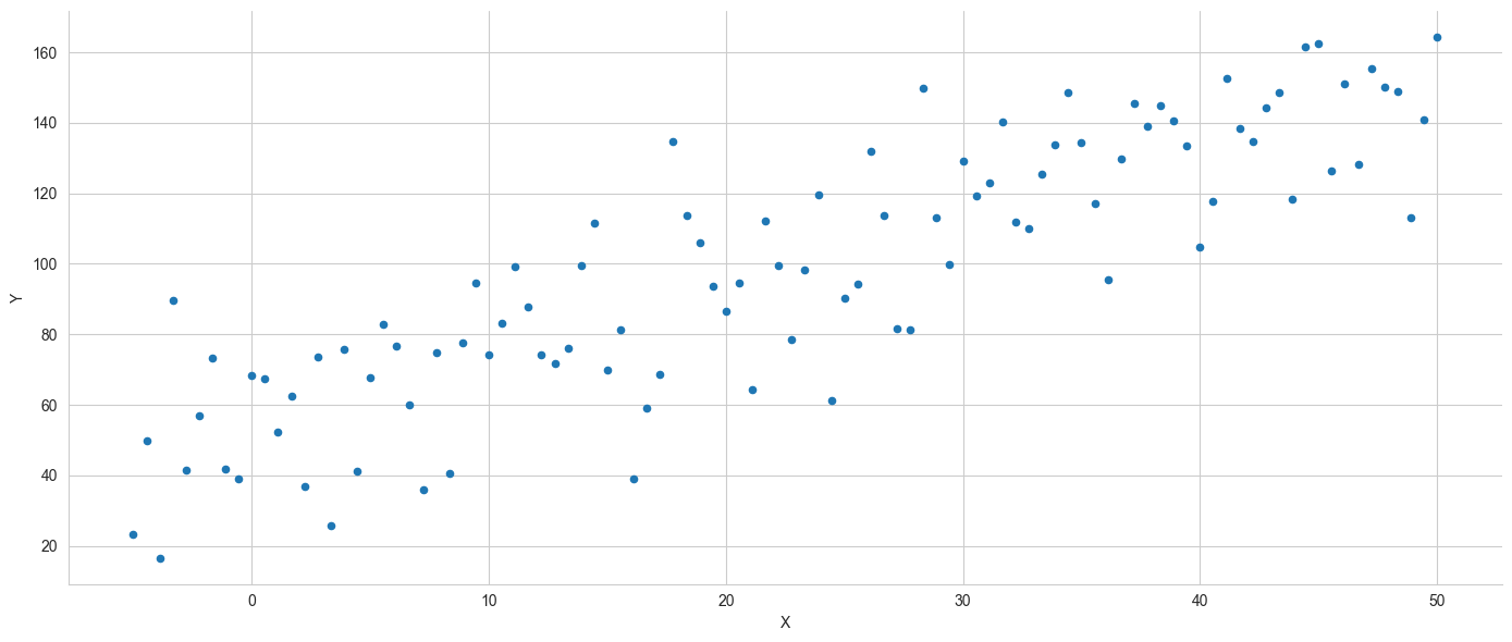
四、拟合
# OLS: Ordinary Least Squares
X = sm.add_constant(data['X'])
model = sm.OLS(data['Y'], X).fit()
print(model.summary())
打印模型结果:
                            OLS Regression Results
==============================================================================
Dep. Variable:                      Y   R-squared:                       0.742
Model:                            OLS   Adj. R-squared:                  0.739
Method:                 Least Squares   F-statistic:                     281.8
Date:                Wed, 17 Sep 2025   Prob (F-statistic):           1.39e-30
Time:                        16:28:00   Log-Likelihood:                -435.02
No. Observations:                 100   AIC:                             874.0
Df Residuals:                      98   BIC:                             879.2
Df Model:                           1
Covariance Type:            nonrobust
==============================================================================coef    std err          t      P>|t|      [0.025      0.975]
------------------------------------------------------------------------------
const         53.8536      3.263     16.503      0.000      47.378      60.330
X              1.9826      0.118     16.786      0.000       1.748       2.217
==============================================================================
Omnibus:                        0.934   Durbin-Watson:                   2.030
Prob(Omnibus):                  0.627   Jarque-Bera (JB):                1.024
Skew:                          -0.213   Prob(JB):                        0.599
Kurtosis:                       2.746   Cond. No.                         47.6
==============================================================================Notes:
[1] Standard Errors assume that the covariance matrix of the errors is correctly specified.
五、模型效果说明
R-squared (coefficient of determination)
0.8: The fitting is very good
0.5~0.8: Medium
< 0.5: Poor fitting
Adj-R ² is almost equal to R ² → no overfitting
Prob (F-statistic) < 0.05, good
A p-value less than 0.05 indicates statistical significance
六、手动公式计算验证
# β̂ = (XᵀX)⁻¹Xᵀy
# Calculate by hand using the OLS formula
beta = np.linalg.inv(X.T.dot(X)).dot(X.T.dot(y))
pd.Series(beta, index=X.columns)
const 53.85
X 1.98
dtype: float64
可以发现,和模型计算出来的差不多。(详细可见我的视频讲解)
七、作图展示
data['y-hat'] = model.predict()
data['residuals'] = model.resid
ax = data.plot.scatter(x='X', y='Y', c='darkgrey', figsize=(14,6))
data.plot.line(x='X', y='y-hat', ax=ax);
# for _, row in data.iterrows():
#     plt.plot((row.X, row.X), (row.Y, row['y-hat']), 'k-')
sns.despine()
plt.tight_layout()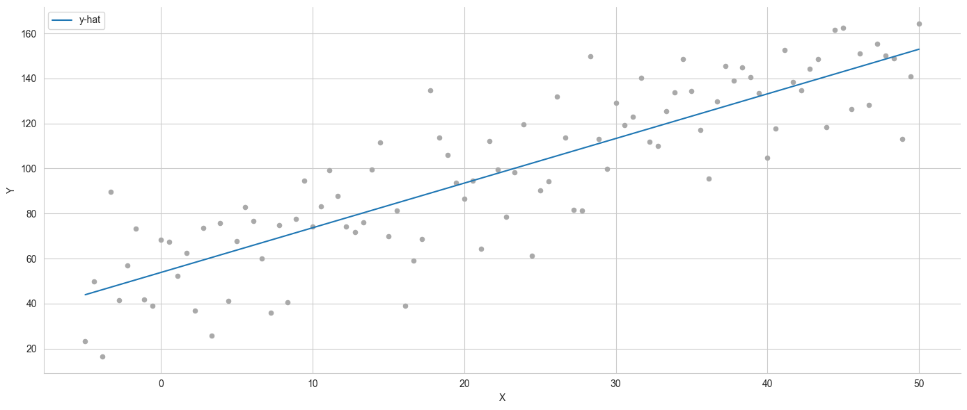
可以发现,基本上是和数据拟合一致的。
# Reference: https://github.com/stefan-jansen/machine-learning-for-trading/blob/main/07_linear_models/01_linear_regression_intro.ipynb