量化交易 - Multiple Regression 多变量线性回归(机器学习)
目录
一、构建数据&作图
二、模型拟合
三、手动验证
四、手动画图
五、更多参数的线性回归
一、构建数据&作图
这里用两个参数
import warnings
warnings.filterwarnings('ignore')
%matplotlib inlineimport numpy as np
import pandas as pdimport matplotlib.pyplot as plt
import seaborn as snsimport statsmodels.api as sm
from sklearn.linear_model import SGDRegressor
from sklearn.preprocessing import StandardScalersns.set_style('whitegrid')
pd.options.display.float_format = '{:,.2f}'.format
## Create data
size = 25
X_1, X_2 = np.meshgrid(np.linspace(-50, 50, size), np.linspace(-50, 50, size), indexing='ij')
data = pd.DataFrame({'X_1': X_1.ravel(), 'X_2': X_2.ravel()})
data['Y'] = 50 + data.X_1 + 3 * data.X_2 + np.random.normal(0, 50, size=size**2)## Plot
# This writing style has been deprecated since version 3.4
# three_dee = plt.figure(figsize=(15, 5)).gca(projection='3d')
fig = plt.figure(figsize=(15, 5))
three_dee = fig.add_subplot(111, projection='3d')
three_dee.scatter(data.X_1, data.X_2, data.Y, c='g')
sns.despine()
plt.tight_layout()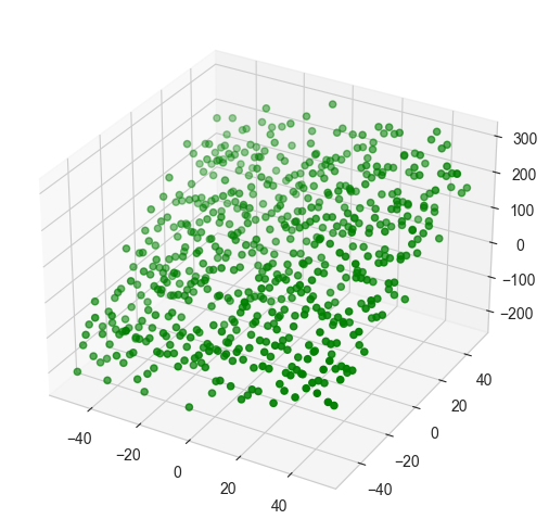
注意:
# This writing style has been deprecated since version 3.4
# three_dee = plt.figure(figsize=(15, 5)).gca(projection='3d')
需要改成:
fig = plt.figure(figsize=(15, 5))
three_dee = fig.add_subplot(111, projection='3d')
二、模型拟合
X = data[['X_1', 'X_2']]
y = data['Y']
X_ols = sm.add_constant(X)
model = sm.OLS(y, X_ols).fit()
print(model.summary())
OLS Regression Results
==============================================================================
Dep. Variable: Y R-squared: 0.780
Model: OLS Adj. R-squared: 0.779
Method: Least Squares F-statistic: 1103.
Date: Wed, 17 Sep 2025 Prob (F-statistic): 2.74e-205
Time: 18:16:55 Log-Likelihood: -3339.4
No. Observations: 625 AIC: 6685.
Df Residuals: 622 BIC: 6698.
Df Model: 2
Covariance Type: nonrobust
==============================================================================coef std err t P>|t| [0.025 0.975]
------------------------------------------------------------------------------
const 48.9968 2.029 24.144 0.000 45.012 52.982
X_1 0.9752 0.068 14.438 0.000 0.843 1.108
X_2 3.0190 0.068 44.699 0.000 2.886 3.152
==============================================================================
Omnibus: 4.056 Durbin-Watson: 1.851
Prob(Omnibus): 0.132 Jarque-Bera (JB): 3.384
Skew: -0.085 Prob(JB): 0.184
Kurtosis: 2.682 Cond. No. 30.0
==============================================================================Notes:
[1] Standard Errors assume that the covariance matrix of the errors is correctly specified.三、手动验证
# β̂ = (XᵀX)⁻¹Xᵀy
# Calculate by hand using the OLS formula
beta = np.linalg.inv(X_ols.T.dot(X_ols)).dot(X_ols.T.dot(y))
pd.Series(beta, index=X_ols.columns)
const 49.00
X_1 0.98
X_2 3.02
dtype: float64四、手动画图
# This writing style has been deprecated since version 3.4
# three_dee = plt.figure(figsize=(15, 5)).gca(projection='3d')
fig = plt.figure(figsize=(15, 5))
three_dee = fig.add_subplot(111, projection='3d')
three_dee.scatter(data.X_1, data.X_2, data.Y, c='g')
data['y-hat'] = model.predict()
to_plot = data.set_index(['X_1', 'X_2']).unstack().loc[:, 'y-hat']
three_dee.plot_surface(X_1, X_2, to_plot.values, color='black', alpha=0.2, linewidth=1, antialiased=True)
# for _, row in data.iterrows():
#     plt.plot((row.X_1, row.X_1), (row.X_2, row.X_2), (row.Y, row['y-hat']), 'k-');
three_dee.set_xlabel('$X_1$');three_dee.set_ylabel('$X_2$');three_dee.set_zlabel('$Y, \hat{Y}$')
sns.despine()
plt.tight_layout()
# we can see it's a plane.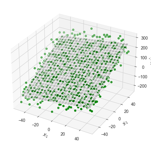
五、更多参数的线性回归
# We can not draw it on the graph, if there are more than 3 parameters.import numpy as np
import pandas as pd
import statsmodels.api as sm# --------------------------------------------------
# 1. Simulate a 4-parameter linear model (not including β0)
#    Y = β0 + β1*X1 + β2*X2 + β3*X3 + β4*X4 + ε
# --------------------------------------------------
n = 10000                                 # sample size
np.random.seed(42)# design matrix (4 explanatory variables)
X = pd.DataFrame({'X_1': np.random.normal(0, 10, n),'X_2': np.random.normal(5, 3, n),'X_3': np.random.normal(-2, 7, n),'X_4': np.random.uniform(-50, 50, n)
})# true coefficients
true_beta = np.array([50, 1.0, -2.0, 3.0, -4.0])   # [β0, β1, β2, β3, β4]# add intercept term and generate response
X_ols = sm.add_constant(X)            # adds β0 column
y = X_ols @ true_beta + np.random.normal(0, 25, n)# --------------------------------------------------
# 2. Fit OLS with statsmodels
# --------------------------------------------------
model = sm.OLS(y, X_ols).fit()# --------------------------------------------------
# 3. Display results
# --------------------------------------------------
print(model.summary())
内容:
                            OLS Regression Results
==============================================================================
Dep. Variable:                      y   R-squared:                       0.958
Model:                            OLS   Adj. R-squared:                  0.958
Method:                 Least Squares   F-statistic:                 5.675e+04
Date:                Wed, 17 Sep 2025   Prob (F-statistic):               0.00
Time:                        18:16:56   Log-Likelihood:                -46325.
No. Observations:               10000   AIC:                         9.266e+04
Df Residuals:                    9995   BIC:                         9.270e+04
Df Model:                           4
Covariance Type:            nonrobust
==============================================================================coef    std err          t      P>|t|      [0.025      0.975]
------------------------------------------------------------------------------
const         50.3440      0.494    101.993      0.000      49.376      51.312
X_1            1.0193      0.025     41.101      0.000       0.971       1.068
X_2           -2.0505      0.083    -24.743      0.000      -2.213      -1.888
X_3            2.9489      0.036     82.207      0.000       2.879       3.019
X_4           -4.0003      0.009   -466.805      0.000      -4.017      -3.984
==============================================================================
Omnibus:                        2.003   Durbin-Watson:                   1.989
Prob(Omnibus):                  0.367   Jarque-Bera (JB):                2.020
Skew:                          -0.034   Prob(JB):                        0.364
Kurtosis:                       2.986   Cond. No.                         58.2
==============================================================================Notes:
[1] Standard Errors assume that the covariance matrix of the errors is correctly specified.
手动验证:
# --------------------------------------------------
# 4. Manual β estimate (X'X)^-1 X'y
# --------------------------------------------------
beta = np.linalg.inv(X_ols.T.dot(X_ols)).dot(X_ols.T.dot(y))
pd.Series(beta, index=X_ols.columns)
const 50.34
X_1 1.02
X_2 -2.05
X_3 2.95
X_4 -4.00
dtype: float64# reference: https://github.com/stefan-jansen/machine-learning-for-trading/blob/main/07_linear_models/01_linear_regression_intro.ipynb