SciPy科学计算与应用:SciPy应用实战-数据分析与工程计算
SciPy案例研究:从理论到实践
学习目标
通过本课程,学员将了解一系列实际案例,深入探讨SciPy库在数据分析、物理模拟和工程计算中的应用。同时学员将学习如何利用SciPy解决实际问题,加深对SciPy各个模块的理解和应用能力。
相关知识点
- SciPy案例研究
学习内容
1 SciPy案例研究
1.1 SciPy在数据分析中的应用
1.1.1 数据预处理与统计分析
在数据分析中,数据预处理是一个非常重要的步骤,它包括数据清洗、数据转换和数据归一化等。SciPy提供了丰富的工具来帮助完成这些任务。例如,scipy.stats模块提供了多种统计函数,可以用来计算数据的描述性统计量,如均值、中位数、标准差等。
代码示例:
import numpy as np
from scipy import stats# 生成随机数据
data = np.random.randn(1000)# 计算描述性统计量
mean = np.mean(data)
median = np.median(data)
std_dev = np.std(data)
variance = np.var(data)# 输出结果
print(f"Mean: {mean}")
print(f"Median: {median}")
print(f"Standard Deviation: {std_dev}")
print(f"Variance: {variance}")# 检验数据是否符合正态分布
k2, p = stats.normaltest(data)
alpha = 1e-3
print(f"p = {p}")
if p < alpha:print("The null hypothesis can be rejected")
else:print("The null hypothesis cannot be rejected")
Mean: 0.02420189499899693
Median: -0.014486221982463464
Standard Deviation: 0.96647641874594
Variance: 0.9340766679919775
p = 0.027943475815425552
The null hypothesis cannot be rejected
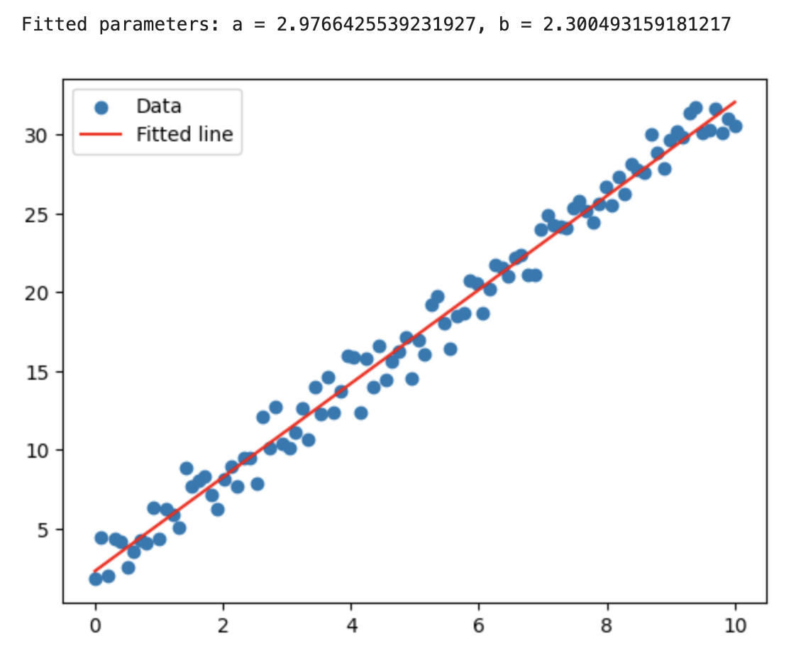
1.1.2 数据拟合与回归分析
数据拟合是数据分析中的另一个重要环节,它可以帮助理解数据之间的关系。SciPy的scipy.optimize模块提供了多种优化算法,可以用来进行线性回归、多项式拟合等。
代码示例:
import numpy as np
from scipy.optimize import curve_fit
import matplotlib.pyplot as plt# 生成模拟数据
x = np.linspace(0, 10, 100)
y = 3 * x + 2 + np.random.normal(0, 1, 100)# 定义线性模型
def linear_model(x, a, b):return a * x + b# 拟合数据
params, _ = curve_fit(linear_model, x, y)# 输出拟合参数
print(f"Fitted parameters: a = {params[0]}, b = {params[1]}")# 绘制拟合结果
plt.scatter(x, y, label='Data')
plt.plot(x, linear_model(x, *params), 'r', label='Fitted line')
plt.legend()
plt.show()
1.2 物理模拟中的SciPy
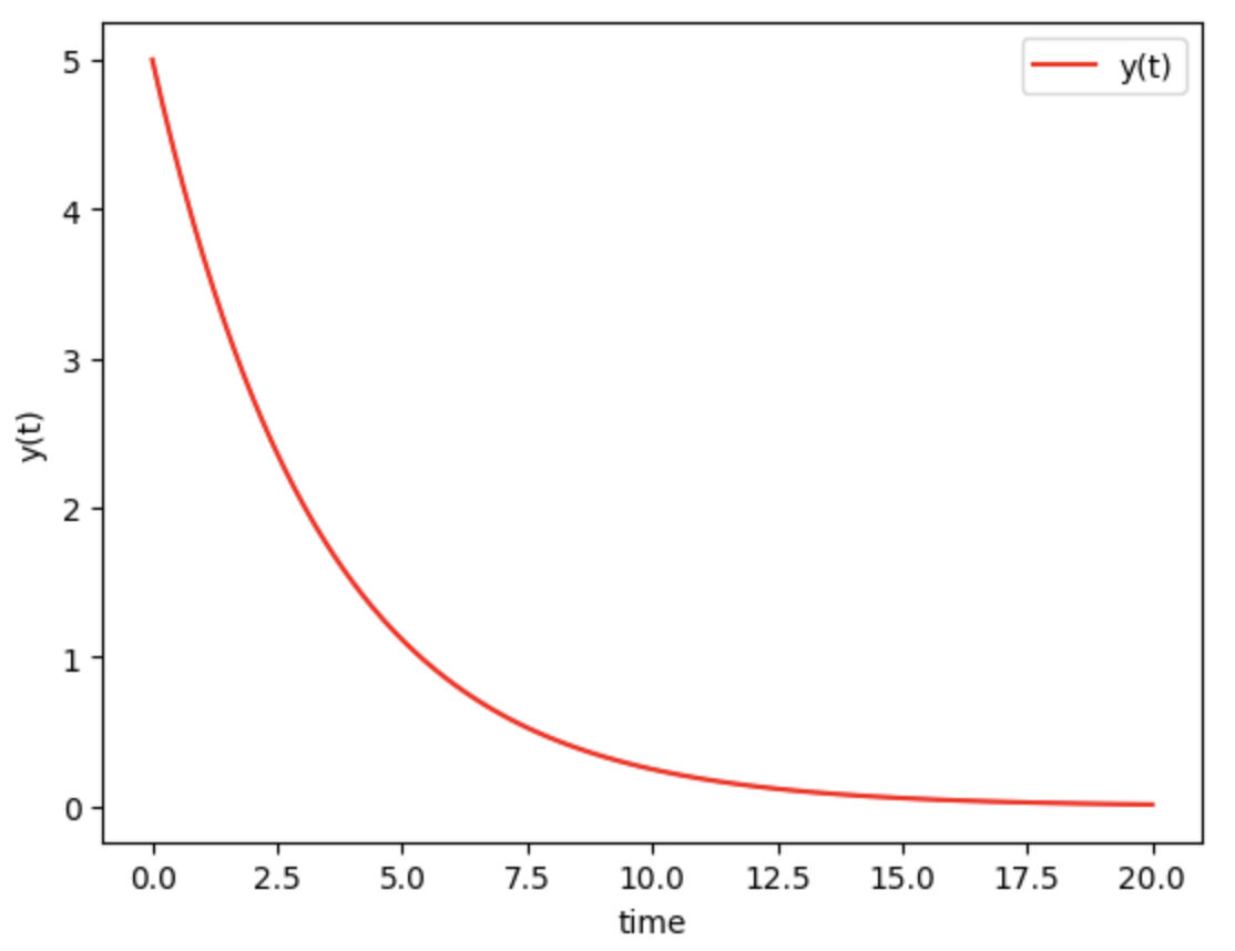
1.2.1 常微分方程的数值解
在物理模拟中,常微分方程(ODE)的数值解是一个常见的问题。SciPy的scipy.integrate模块提供了多种求解ODE的方法,如odeint和solve_ivp。
代码示例:
import numpy as np
from scipy.integrate import odeint
import matplotlib.pyplot as plt# 定义常微分方程
def model(y, t):k = 0.3dydt = -k * yreturn dydt# 初始条件
y0 = 5# 时间点
t = np.linspace(0, 20, 100)# 求解ODE
y = odeint(model, y0, t)# 绘制结果
plt.plot(t, y, 'r', label='y(t)')
plt.xlabel('time')
plt.ylabel('y(t)')
plt.legend()
plt.show()
1.2 物理模拟中的SciPy
1.2.1 常微分方程的数值解
在物理模拟中,常微分方程(ODE)的数值解是一个常见的问题。SciPy的scipy.integrate模块提供了多种求解ODE的方法,如odeint和solve_ivp。
代码示例:
 import numpy as np
from scipy.integrate import odeint
import matplotlib.pyplot as plt# 定义常微分方程
def model(y, t):k = 0.3dydt = -k * yreturn dydt# 初始条件
y0 = 5# 时间点
t = np.linspace(0, 20, 100)# 求解ODE
y = odeint(model, y0, t)# 绘制结果
plt.plot(t, y, 'r', label='y(t)')
plt.xlabel('time')
plt.ylabel('y(t)')
plt.legend()
plt.show()
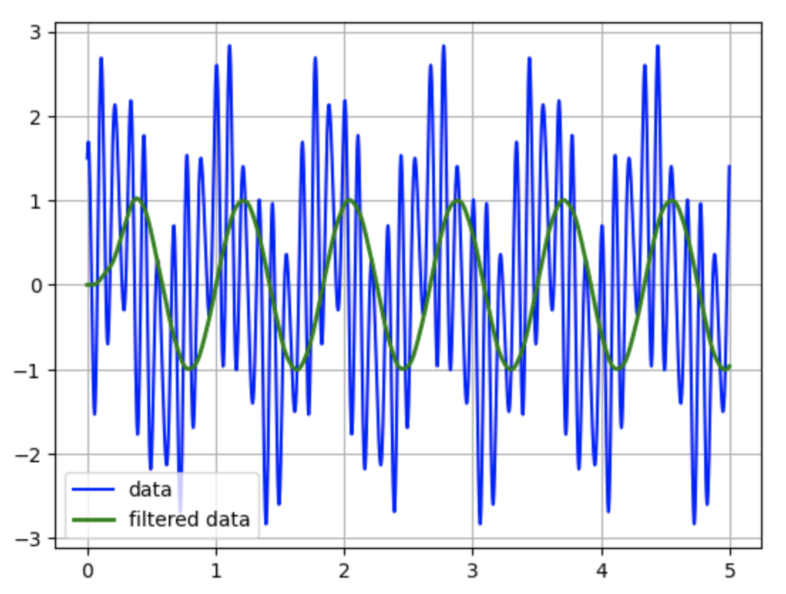
1.2.2 信号处理
在物理模拟中,信号处理是一个重要的领域。SciPy的scipy.signal模块提供了多种信号处理工具,如滤波器设计、频谱分析等。
代码示例:
import numpy as np
from scipy.signal import butter, lfilter, freqz
import matplotlib.pyplot as plt# 定义Butterworth滤波器
def butter_lowpass(cutoff, fs, order=5):nyq = 0.5 * fsnormal_cutoff = cutoff / nyqb, a = butter(order, normal_cutoff, btype='low', analog=False)return b, adef butter_lowpass_filter(data, cutoff, fs, order=5):b, a = butter_lowpass(cutoff, fs, order=order)y = lfilter(b, a, data)return y# 生成模拟信号
fs = 500.0
T = 5.0
n = int(T * fs)
t = np.linspace(0, T, n, endpoint=False)
data = np.sin(1.2 * 2 * np.pi * t) + 1.5 * np.cos(9 * 2 * np.pi * t) + 0.5 * np.sin(12.0 * 2 * np.pi * t)# 滤波器参数
cutoff = 3.667
order = 6# 应用滤波器
y = butter_lowpass_filter(data, cutoff, fs, order)# 绘制结果
plt.plot(t, data, 'b-', label='data')
plt.plot(t, y, 'g-', linewidth=2, label='filtered data')
plt.legend()
plt.grid(True)
plt.show()
1.3 工程计算中的SciPy
1.3.1 优化问题
在工程计算中,优化问题是一个常见的任务。SciPy的scipy.optimize模块提供了多种优化算法,如最小化、最大化、约束优化等。
代码示例:
import numpy as np
from scipy.optimize import minimize# 定义目标函数
def objective(x):return x[0]**2 + x[1]**2# 定义约束条件
def constraint1(x):return x[0] * x[1] - 1# 初始猜测
x0 = [1, 1]# 定义约束
con1 = {'type': 'eq', 'fun': constraint1}# 求解优化问题
solution = minimize(objective, x0, method='SLSQP', constraints=[con1])# 输出结果
print(f"Optimal solution: x = {solution.x}")
print(f"Optimal value: f(x) = {solution.fun}")
Optimal solution: x = [1. 1.]
Optimal value: f(x) = 2.0
1.3.2 线性代数
在工程计算中,线性代数是一个基础且重要的领域。SciPy的scipy.linalg模块提供了多种线性代数工具,如矩阵求逆、特征值分解等。
代码示例:
import numpy as np
from scipy.linalg import inv, eig# 定义矩阵
A = np.array([[4, 2], [1, 3]])# 求逆矩阵
A_inv = inv(A)# 计算特征值和特征向量
eigenvalues, eigenvectors = eig(A)# 输出结果
print(f"Inverse of A: \n{A_inv}")
print(f"Eigenvalues of A: \n{eigenvalues}")
print(f"Eigenvectors of A: \n{eigenvectors}")
Inverse of A:
[[ 0.3 -0.2][-0.1  0.4]]
Eigenvalues of A:
[5.+0.j 2.+0.j]
Eigenvectors of A:
[[ 0.89442719 -0.70710678][ 0.4472136   0.70710678]]
通过本课程,学员将能够熟练掌握SciPy在数据分析、物理模拟和工程计算中的应用,提升解决实际问题的能力。