6月7日day47打卡

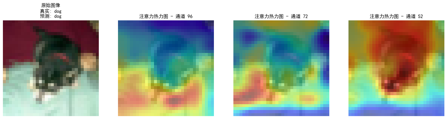
注意力热图可视化

昨天代码中注意力热图的部分顺移至今天

知识点回顾：

热力图

作业：对比不同卷积层热图可视化的结果

import torch
import torch.nn as nn
import torch.optim as optim
from torchvision import datasets, transforms
from torch.utils.data import DataLoader
import matplotlib.pyplot as plt
import numpy as np# 设置中文字体支持
plt.rcParams["font.family"] = ["SimHei"]
plt.rcParams['axes.unicode_minus'] = False  # 解决负号显示问题# 检查GPU是否可用
device = torch.device("cuda" if torch.cuda.is_available() else "cpu")
print(f"使用设备: {device}")# 1. 数据预处理
# 训练集：使用多种数据增强方法提高模型泛化能力
train_transform = transforms.Compose([# 随机裁剪图像，从原图中随机截取32x32大小的区域transforms.RandomCrop(32, padding=4),# 随机水平翻转图像（概率0.5）transforms.RandomHorizontalFlip(),# 随机颜色抖动：亮度、对比度、饱和度和色调随机变化transforms.ColorJitter(brightness=0.2, contrast=0.2, saturation=0.2, hue=0.1),# 随机旋转图像（最大角度15度）transforms.RandomRotation(15),# 将PIL图像或numpy数组转换为张量transforms.ToTensor(),# 标准化处理：每个通道的均值和标准差，使数据分布更合理transforms.Normalize((0.4914, 0.4822, 0.4465), (0.2023, 0.1994, 0.2010))
])# 测试集：仅进行必要的标准化，保持数据原始特性，标准化不损失数据信息，可还原
test_transform = transforms.Compose([transforms.ToTensor(),transforms.Normalize((0.4914, 0.4822, 0.4465), (0.2023, 0.1994, 0.2010))
])# 2. 加载CIFAR-10数据集
train_dataset = datasets.CIFAR10(root='./data',train=True,download=True,transform=train_transform  # 使用增强后的预处理
)test_dataset = datasets.CIFAR10(root='./data',train=False,transform=test_transform  # 测试集不使用增强
)# 3. 创建数据加载器
batch_size = 64
train_loader = DataLoader(train_dataset, batch_size=batch_size, shuffle=True)
test_loader = DataLoader(test_dataset, batch_size=batch_size, shuffle=False)# ===================== 新增：通道注意力模块（SE模块） =====================
class ChannelAttention(nn.Module):"""通道注意力模块(Squeeze-and-Excitation)"""def __init__(self, in_channels, reduction_ratio=16):"""参数:in_channels: 输入特征图的通道数reduction_ratio: 降维比例，用于减少参数量"""super(ChannelAttention, self).__init__()# 全局平均池化 - 将空间维度压缩为1x1，保留通道信息self.avg_pool = nn.AdaptiveAvgPool2d(1)# 全连接层 + 激活函数，用于学习通道间的依赖关系self.fc = nn.Sequential(# 降维：压缩通道数，减少计算量nn.Linear(in_channels, in_channels // reduction_ratio, bias=False),nn.ReLU(inplace=True),# 升维：恢复原始通道数nn.Linear(in_channels // reduction_ratio, in_channels, bias=False),# Sigmoid将输出值归一化到[0,1]，表示通道重要性权重nn.Sigmoid())def forward(self, x):"""参数:x: 输入特征图，形状为 [batch_size, channels, height, width]返回:加权后的特征图，形状不变"""batch_size, channels, height, width = x.size()# 1. 全局平均池化：[batch_size, channels, height, width] → [batch_size, channels, 1, 1]avg_pool_output = self.avg_pool(x)# 2. 展平为一维向量：[batch_size, channels, 1, 1] → [batch_size, channels]avg_pool_output = avg_pool_output.view(batch_size, channels)# 3. 通过全连接层学习通道权重：[batch_size, channels] → [batch_size, channels]channel_weights = self.fc(avg_pool_output)# 4. 重塑为二维张量：[batch_size, channels] → [batch_size, channels, 1, 1]channel_weights = channel_weights.view(batch_size, channels, 1, 1)# 5. 将权重应用到原始特征图上（逐通道相乘）return x * channel_weights  # 输出形状：[batch_size, channels, height, width]class CNN(nn.Module):def __init__(self):super(CNN, self).__init__()  # ---------------------- 第一个卷积块 ----------------------self.conv1 = nn.Conv2d(3, 32, 3, padding=1)self.bn1 = nn.BatchNorm2d(32)self.relu1 = nn.ReLU()# 新增：插入通道注意力模块（SE模块）self.ca1 = ChannelAttention(in_channels=32, reduction_ratio=16)  self.pool1 = nn.MaxPool2d(2, 2)  # ---------------------- 第二个卷积块 ----------------------self.conv2 = nn.Conv2d(32, 64, 3, padding=1)self.bn2 = nn.BatchNorm2d(64)self.relu2 = nn.ReLU()# 新增：插入通道注意力模块（SE模块）self.ca2 = ChannelAttention(in_channels=64, reduction_ratio=16)  self.pool2 = nn.MaxPool2d(2)  # ---------------------- 第三个卷积块 ----------------------self.conv3 = nn.Conv2d(64, 128, 3, padding=1)self.bn3 = nn.BatchNorm2d(128)self.relu3 = nn.ReLU()# 新增：插入通道注意力模块（SE模块）self.ca3 = ChannelAttention(in_channels=128, reduction_ratio=16)  self.pool3 = nn.MaxPool2d(2)  # ---------------------- 全连接层（分类器） ----------------------self.fc1 = nn.Linear(128 * 4 * 4, 512)self.dropout = nn.Dropout(p=0.5)self.fc2 = nn.Linear(512, 10)def forward(self, x):# ---------- 卷积块1处理 ----------x = self.conv1(x)       x = self.bn1(x)         x = self.relu1(x)       x = self.ca1(x)  # 应用通道注意力x = self.pool1(x)       # ---------- 卷积块2处理 ----------x = self.conv2(x)       x = self.bn2(x)         x = self.relu2(x)       x = self.ca2(x)  # 应用通道注意力x = self.pool2(x)       # ---------- 卷积块3处理 ----------x = self.conv3(x)       x = self.bn3(x)         x = self.relu3(x)       x = self.ca3(x)  # 应用通道注意力x = self.pool3(x)       # ---------- 展平与全连接层 ----------x = x.view(-1, 128 * 4 * 4)  x = self.fc1(x)           x = self.relu3(x)         x = self.dropout(x)       x = self.fc2(x)           return x  # 重新初始化模型，包含通道注意力模块
model = CNN()
model = model.to(device)  # 将模型移至GPU（如果可用）criterion = nn.CrossEntropyLoss()  # 交叉熵损失函数
optimizer = optim.Adam(model.parameters(), lr=0.001)  # Adam优化器# 引入学习率调度器，在训练过程中动态调整学习率--训练初期使用较大的 LR 快速降低损失，训练后期使用较小的 LR 更精细地逼近全局最优解。
# 在每个 epoch 结束后，需要手动调用调度器来更新学习率，可以在训练过程中调用 scheduler.step()
scheduler = optim.lr_scheduler.ReduceLROnPlateau(optimizer,        # 指定要控制的优化器（这里是Adam）mode='min',       # 监测的指标是"最小化"（如损失函数）patience=3,       # 如果连续3个epoch指标没有改善，才降低LRfactor=0.5        # 降低LR的比例（新LR = 旧LR × 0.5）
)def visualize_feature_maps(model, test_loader, device, layer_names, num_images=3, num_channels=9):"""可视化指定层的特征图（修复循环冗余问题）参数:model: 模型test_loader: 测试数据加载器device: 设备（如'cuda'或'cpu'）layer_names: 要可视化的层名称（如['conv1', 'conv2', 'conv3']）num_images: 可视化的图像总数num_channels: 每个图像显示的通道数（取前num_channels个通道）"""model.eval()  # 设置为评估模式class_names = ['飞机', '汽车', '鸟', '猫', '鹿', '狗', '青蛙', '马', '船', '卡车']# 从测试集加载器中提取指定数量的图像（避免嵌套循环）# 初始化空列表，用于暂存从测试数据加载器中获取的图像批量和标签批量images_list, labels_list = [], []# 遍历测试数据加载器（每次迭代获取一个批量的图像和标签）for images, labels in test_loader:# 将当前批量的图像张量添加到images_list列表中images_list.append(images)# 将当前批量的标签张量添加到labels_list列表中labels_list.append(labels)# 终止条件：当已收集的批量数 × 每个批量的大小 ≥ 需要的总图像数时，停止收集# （例如：batch_size=64，num_images=5 → 第一个批量就满足64≥5，循环仅执行1次）if len(images_list) * test_loader.batch_size >= num_images:break # 退出循环，避免收集多余数据# 拼接并截取到目标数量images = torch.cat(images_list, dim=0)[:num_images].to(device)labels = torch.cat(labels_list, dim=0)[:num_images].to(device)with torch.no_grad():# 存储各层特征图feature_maps = {}# 保存钩子句柄hooks = []# 定义钩子函数，捕获指定层的输出def hook(module, input, output, name):feature_maps[name] = output.cpu()  # 保存特征图到字典# 为每个目标层注册钩子，并保存钩子句柄# 遍历需要可视化的层名称列表（如['conv1', 'conv2', 'conv3']）for name in layer_names:# 从模型中获取当前层名对应的模块（例如name='conv1'时，module=model.conv1）module = getattr(model, name)# 为当前层注册前向钩子（forward hook）：模型前向传播时，钩子会触发hook函数捕获输出# lambda中n=name：固定当前循环的层名（避免闭包延迟绑定问题，确保每个钩子对应正确层名）hook_handle = module.register_forward_hook(lambda m, i, o, n=name: hook(m, i, o, n))# 保存钩子句柄到列表（后续通过句柄移除钩子，避免内存泄漏）hooks.append(hook_handle)# 前向传播触发钩子_ = model(images)# 正确移除钩子for hook_handle in hooks:hook_handle.remove()# 可视化每个图像的各层特征图（仅一层循环）# 遍历所有需要可视化的测试图像（共num_images张）for img_idx in range(num_images):# 从GPU（或CPU）中取出第img_idx张图像，调整通道顺序并转为numpy数组# permute(1, 2, 0)：将张量形状从[C, H, W] → [H, W, C]（符合图像显示的通道顺序）img = images[img_idx].cpu().permute(1, 2, 0).numpy()# 反标准化处理（恢复训练前的原始像素值）# 原始标准化公式：img = (img - mean) / std → 反标准化：img = img * std + meanimg = img * np.array([0.2023, 0.1994, 0.2010]).reshape(1, 1, 3) + np.array([0.4914, 0.4822, 0.4465]).reshape(1, 1, 3)img = np.clip(img, 0, 1)  # 确保像素值在[0,1]范围内（避免计算误差导致越界）# 创建子图布局：1行（水平排列），列数=层数+1（原始图像占1列，每层特征图占1列num_layers = len(layer_names)  # 获取需要可视化的层数（如3层）fig, axes = plt.subplots(1, num_layers + 1, figsize=(4 * (num_layers + 1), 4))  # 总宽度随层数动态调整# 显示原始图像axes[0].imshow(img)  # 在第1个子图显示反标准化后的原始图像axes[0].set_title(f'原始图像\n类别: {class_names[labels[img_idx]]}')  # 设置标题（包含真实类别）axes[0].axis('off')  # 关闭坐标轴，仅显示图像# 显示各层特征图（后续每列对应一个层）for layer_idx, layer_name in enumerate(layer_names):# 从特征图字典中获取当前层（如conv1）对应第img_idx张图像的特征图fm = feature_maps[layer_name][img_idx]  # 形状：[num_channels, H, W]fm = fm[:num_channels]  # 仅取前num_channels个通道（如前9个）# 计算小网格的行数和列数（例如num_channels=9 → 3行3列）num_rows = int(np.sqrt(num_channels))  # 行数=通道数的平方根（向下取整）num_cols = num_channels // num_rows if num_rows != 0 else 1  # 列数=通道数//行数（避免除0）# 获取当前层对应的子图位置（第layer_idx+1列）layer_ax = axes[layer_idx + 1]layer_ax.set_title(f'{layer_name}特征图 \n')  # 设置大子图标题（换行使文字更清晰）layer_ax.axis('off')  # 关闭大子图的坐标轴（仅显示内部小网格）# 在大子图内创建小网格（每个小网格显示一个通道的特征图）for ch_idx, channel in enumerate(fm):# 计算小网格在大子图中的位置（归一化坐标）# ch_idx % num_cols：列索引（0~num_cols-1）# (num_rows - 1 - ch_idx // num_cols)：行索引（从上到下排列）# 1/num_cols, 1/num_rows：小网格的宽度和高度（占大子图的1/列数和1/行数）ax = layer_ax.inset_axes([ch_idx % num_cols / num_cols, (num_rows - 1 - ch_idx // num_cols) / num_rows, 1/num_cols, 1/num_rows])ax.imshow(channel.numpy(), cmap='viridis')  # 显示特征图（使用蓝绿黄渐变颜色映射）ax.set_title(f'通道 {ch_idx + 1}')  # 设置小网格标题（通道号从1开始）ax.axis('off')  # 关闭小网格的坐标轴plt.tight_layout()  # 自动调整子图间距，避免重叠plt.show()  # 显示当前图像的所有子图# 调用示例（按需修改参数）
# 定义要可视化的目标层名称列表（选择模型中的三个卷积层）
layer_names = ['conv1', 'conv2', 'conv3']
# 调用特征图可视化函数，触发可视化流程
visualize_feature_maps(model=model,                  # 传入已训练好的模型（用于获取各层特征图）test_loader=test_loader,      # 传入测试数据加载器（用于获取待可视化的测试图像）device=device,                # 指定计算设备（与模型所在设备一致，确保数据和模型在同一设备）layer_names=layer_names,      # 指定要可视化的层列表（使用上面定义的layer_names）num_images=5,                 # 可视化5张测试图像（输出5张大图，每张图对应1张测试图像）num_channels=9                # 每张图像显示前9个通道的特征图（取每个层的前9个通道）)# 可视化空间注意力热力图（显示模型关注的图像区域）
def visualize_attention_map(model, test_loader, device, class_names, num_samples=3):"""可视化模型的注意力热力图，展示模型关注的图像区域"""model.eval()  # 设置为评估模式with torch.no_grad():for i, (images, labels) in enumerate(test_loader):if i >= num_samples:  # 只可视化前几个样本breakimages, labels = images.to(device), labels.to(device)# 创建一个钩子，捕获中间特征图activation_maps = []def hook(module, input, output):activation_maps.append(output.cpu())# 为最后一个卷积层注册钩子（获取特征图）hook_handle = model.conv3.register_forward_hook(hook)# 前向传播，触发钩子outputs = model(images)# 移除钩子hook_handle.remove()# 获取预测结果_, predicted = torch.max(outputs, 1)# 获取原始图像img = images[0].cpu().permute(1, 2, 0).numpy()# 反标准化处理img = img * np.array([0.2023, 0.1994, 0.2010]).reshape(1, 1, 3) + np.array([0.4914, 0.4822, 0.4465]).reshape(1, 1, 3)img = np.clip(img, 0, 1)# 获取激活图（最后一个卷积层的输出）feature_map = activation_maps[0][0].cpu()  # 取第一个样本# 计算通道注意力权重（使用SE模块的全局平均池化）channel_weights = torch.mean(feature_map, dim=(1, 2))  # [C]# 按权重对通道排序sorted_indices = torch.argsort(channel_weights, descending=True)# 创建子图fig, axes = plt.subplots(1, 4, figsize=(16, 4))# 显示原始图像axes[0].imshow(img)axes[0].set_title(f'原始图像\n真实: {class_names[labels[0]]}\n预测: {class_names[predicted[0]]}')axes[0].axis('off')# 显示前3个最活跃通道的热力图for j in range(3):channel_idx = sorted_indices[j]# 获取对应通道的特征图channel_map = feature_map[channel_idx].numpy()# 归一化到[0,1]channel_map = (channel_map - channel_map.min()) / (channel_map.max() - channel_map.min() + 1e-8)# 调整热力图大小以匹配原始图像from scipy.ndimage import zoomheatmap = zoom(channel_map, (32/feature_map.shape[1], 32/feature_map.shape[2]))# 显示热力图axes[j+1].imshow(img)axes[j+1].imshow(heatmap, alpha=0.5, cmap='jet')axes[j+1].set_title(f'注意力热力图 - 通道 {channel_idx}')axes[j+1].axis('off')plt.tight_layout()plt.show()# 调用可视化函数
visualize_attention_map(model, test_loader, device, class_names, num_samples=3)

 

 

@浙大疏锦行​​​​​​​