2025.4.7-2025.4.13文献阅读

摘要

在本周阅读的论文中，作者提出了一种新颖的多图时空注意力模型用于对空气质量的预测。模型通过构建多尺度时空图，包括基于地理距离的距离图、反映直接连接性的邻居图以及捕捉时间因果性的时间因果关系图，从多个维度全面刻画站点间的复杂交互关系。这种多图策略克服了单一图结构在信息表达上的局限性，为后续特征提取提供了丰富的空间信息。同时，作者设计的时空多图注意力融合模块可以巧妙融合站点时间序列的非线性时间相关性与多图的空间信息，通过时间注意力机制和图注意力机制动态调整历史时间步及不同图结构对预测的贡献，并借助门控融合机制自适应平衡时间与空间特征，进一步增强了特征表达能力和模型泛化性。

Abstract

In the paper read this week, the author proposed a novel multi graph spatiotemporal attention model for predicting air quality. The model comprehensively characterizes the complex interaction relationships between sites from multiple dimensions by constructing multi-scale spatiotemporal maps, including distance maps based on geographic distance, neighbor maps reflecting direct connectivity, and temporal causal relationship maps capturing temporal causality. This multi graph strategy overcomes the limitations of a single graph structure in information expression and provides rich spatial information for subsequent feature extraction. At the same time, the spatiotemporal multi graph attention fusion module designed by the author can cleverly integrate the nonlinear temporal correlation of station time series with the spatial information of multiple graphs. Through the temporal attention mechanism and graph attention mechanism, it dynamically adjusts the historical time steps and the contribution of different graph structures to prediction. With the help of gate fusion mechanism, it adaptively balances the temporal and spatial features, further enhancing the feature expression ability and model generalization.

1 文献阅读

本周阅读了一篇名为A multi-graph spatial-temporal attention network for air-quality prediction 的论文

论文链接：A multi-graph spatial-temporal attention network for air-quality prediction

论文中提出的多图时空注意力网络通过构建多尺度时空图、设计时空多图注意力融合模块和时空预测网络，可以有效捕捉站点间的空间和时间关系。论文实验验证了模型在短期和长期空气质量预测任务中的高效性和优越性。

1.1 模型架构

论文提出了一种多图时空注意力网络，用于预测给定区域的空气质量（以PM2.5浓度为指标），其主体框架如下图所示:

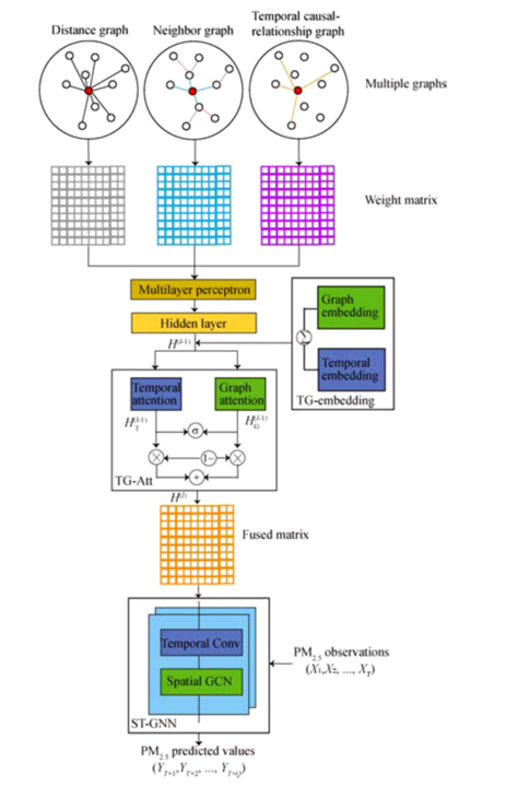
其大体可以分为三个部分，即多尺度时空图的构建、时空多图注意力融合模块以及时空预测网络。其大致的工作流程是先通过历史数据构建三个图，这里的多图构建是论文的一个创新点。通过多层感知机将构建的图映射到Hidden layer并经嵌入处理后通过时空多图注意力融合模块进行特征融合，最后经时空预测网络预测输出对未来时间步的预测。

1.1.1 多尺度时空图的构建

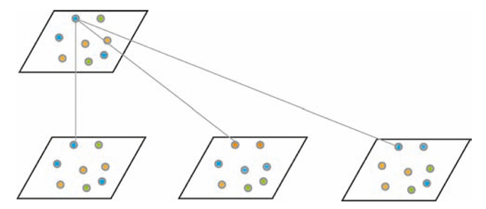
为了全面捕捉站点间的空间和时间关系，模型构造了三种图结构，每种图从不同视角建模站点的交互，分别是距离图、邻居图以及时序因果图。构建多尺度时空图对站点空间信息进行编码的方法结合了多尺度空间距离和时间因果特征，可以更好地从时间和空间维度探索隐藏的空间信息。

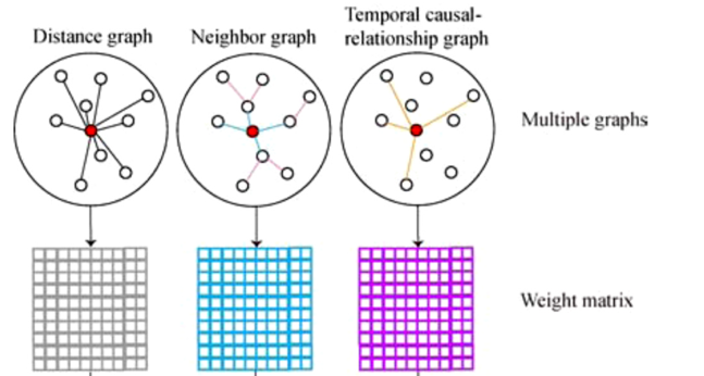
其中距离图反映了站点间地理距离对污染物扩散的影响，它是根据各站点间的距离并经高斯核函数计算边的权重后得到的，它的作用是捕捉空间自相关性，例如污染物通过风向传播的距离依赖；邻居图的构建是为了捕捉站点间的直接连接关系，它可以反映局部空间传播，例如污染物通过直接路径的迁移；一个站点的污染物浓度可能会受到另一个站点的污染物浓度的影响，但有一定的延迟。这说明一个站点的污染物浓度变化会导致另一个站点的污染物浓度也相应变化。时间因果关系图的构建就是为了捕捉站点时间序列间的因果依赖，从而可以知道站点间污染物迁移的时间方向性。

1.1.2 时空多图注意力模块

时空多图注意力模块的作用是为了融合站点时间序列的非线性时间相关性和多图的空间信息。首先模型经过Temporal Multi-Graph Embedding处理将​​时间动态特征​​与​​多图拓扑特征​​编码为统一的嵌入向量。

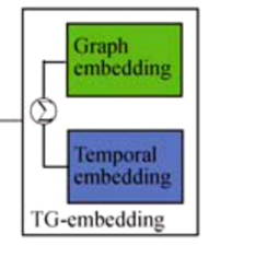
Temporal Multi-Graph Embedding分为时间嵌入和多图嵌入两部分。
时间嵌入将更详细的时间信息编码到向量中，由于区域内不同站点的空气质量预测与自身的非线性时间关系具有很强的相关性，因此在模型中补充更多的时间信息有利于提高预测精度。
时间嵌入仅表示各个站点的非线性相关性。为了进一步捕捉站点之间的关系信息，论文引入了多图嵌入的概念。作者按照所构建的三个图为每个节点分配不同的权重，将不同图中每个节点的权重用作多图嵌入。

最后将时间嵌入t和多图嵌入g逐元素相加得到TG融合嵌入。所得TG融合嵌入作为时空多图注意力模块的输入。
时空多图注意力模块结构如下图所示，其结构大致可以分为三个模块：时间注意力机制、图注意力机制以及门控融合机制。

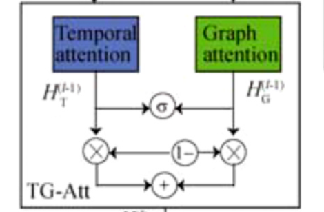
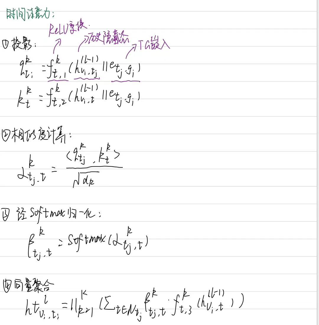
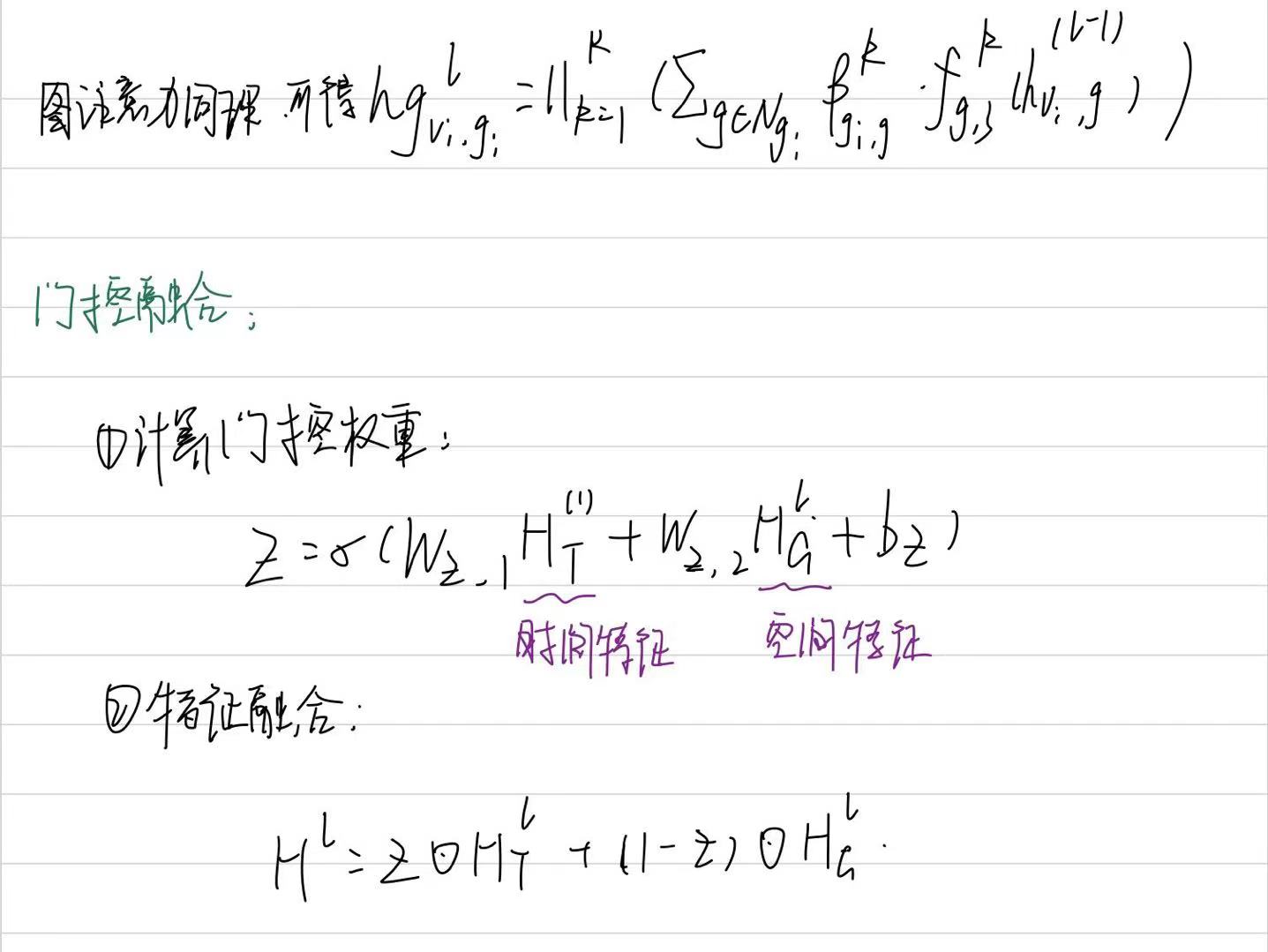
模块通过时间注意力机制捕捉每个站点时间序列在不同时间步间的非线性相关性，从而动态调整历史时间步的影响；通过图注意力机制融合不同图结构中的空间信息从而增强空间特征的多尺度表达。最后通过门控融合机制将时间注意力得到的时间特征与图注意力得到的空间特征相融合，保证时间动态与空间关系的动态平衡。在这里，无论是时间注意力机制还是图注意力机制都是多头注意力。其过程概括如下所示：

1.1.3 时空预测网络

时空预测网络由几个时空卷积块串联组成。每个时空卷积块由一个空间图卷积层和两个门控时间卷积层组成。

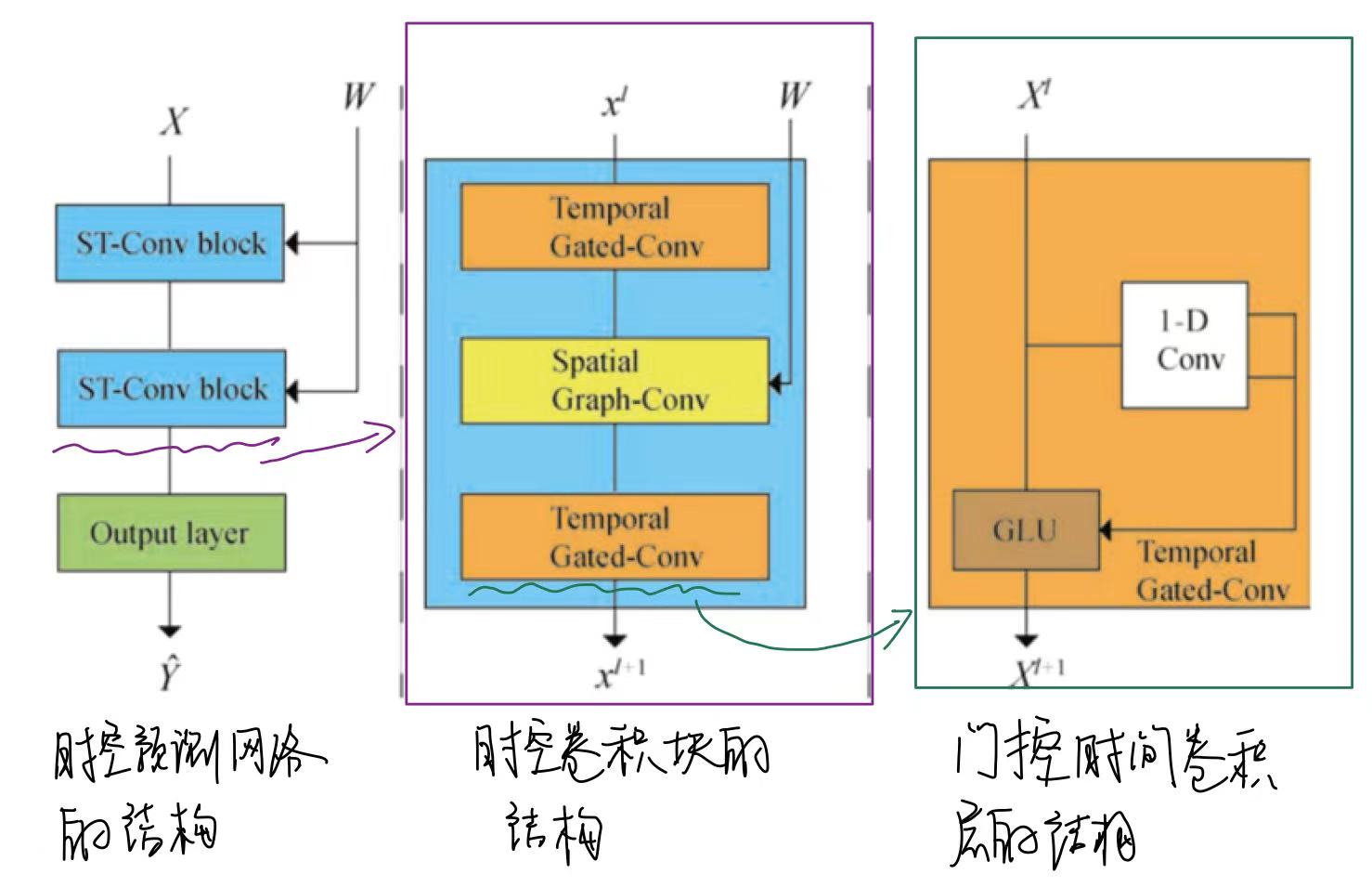
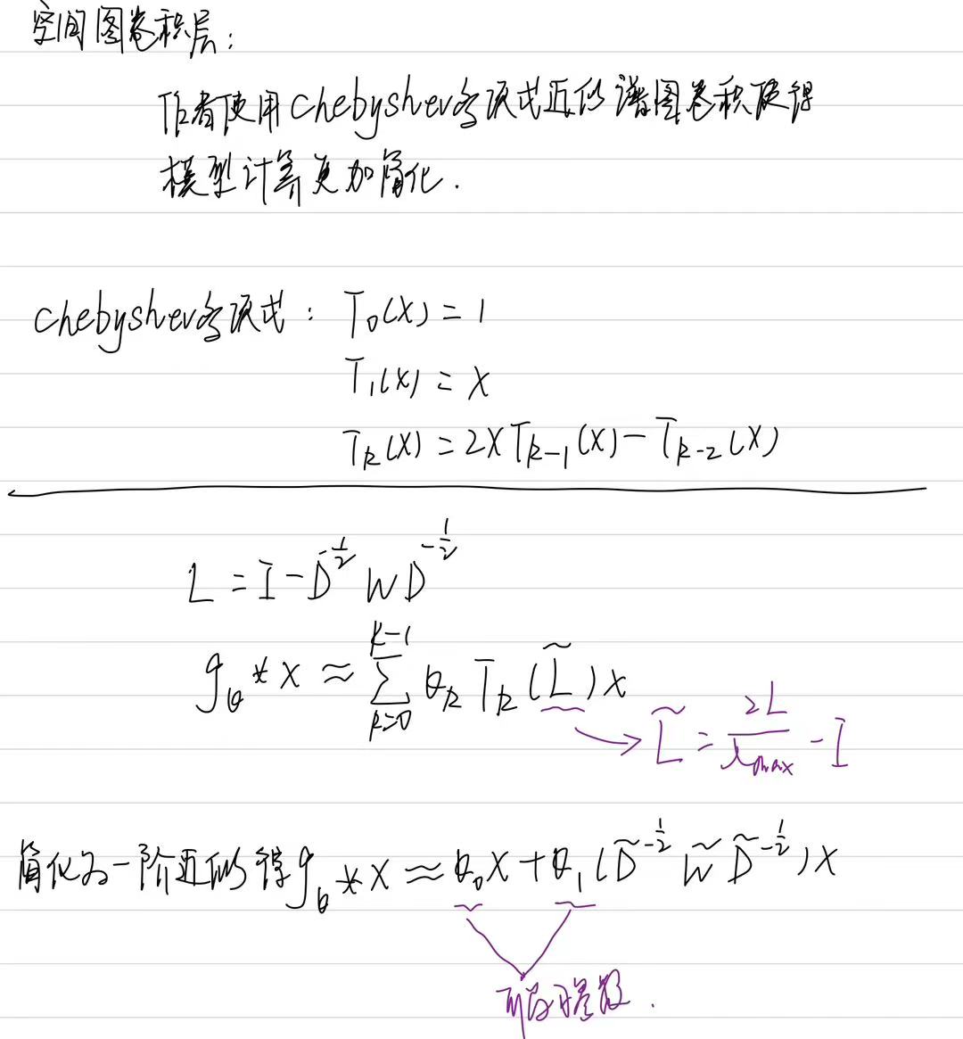
其中，门控时间卷积层使用一维因果卷积和门控线性单元来提取空气质量站网络随时间序列变化的特征，空间图卷积层利用GCN来捕获有关空气质量站网络互连性的空间信息，通过 Chebyshev 多项式近似谱图卷积：

模型的代码实现如下：

import torch
import torch.nn as nn
import torch.nn.functional as F
import dgl
from dgl.nn.pytorch import GraphConv
import numpy as np
from scipy.spatial.distance import pdist, squareform

def build_distance_graph(coords, sigma_D=1000, epsilon=0.3):
    """
    Build a distance graph based on geographical coordinates using a Gaussian kernel.
    
    Parameters:
    - coords: numpy array of shape (N, 2), where N is the number of stations (latitude, longitude).
    - sigma_D: standard deviation for the Gaussian kernel.
    - epsilon: threshold to enforce sparsity in the adjacency matrix.
    
    Returns:
    - W_D: adjacency matrix for the distance graph (numpy array of shape (N, N)).
    """
    # Compute pairwise Euclidean distances between all stations
    dist_matrix = squareform(pdist(coords, metric='euclidean'))
    # Apply Gaussian kernel to convert distances to weights
    W_D = np.exp(- (dist_matrix ** 2) / (sigma_D ** 2))
    # Apply sparsity threshold
    W_D[W_D < epsilon] = 0
    # Remove self-loops by setting diagonal to zero
    np.fill_diagonal(W_D, 0)
    return W_D

def build_neighbor_graph(coords, k=5):
    """
    Build a neighbor graph based on k-nearest neighbors.
    
    Parameters:
    - coords: numpy array of shape (N, 2), where N is the number of stations.
    - k: number of nearest neighbors to connect for each node.
    
    Returns:
    - W_N: adjacency matrix for the neighbor graph (numpy array of shape (N, N)).
    """
    # Compute pairwise Euclidean distances
    dist_matrix = squareform(pdist(coords, metric='euclidean'))
    # Get indices of k nearest neighbors (excluding self)
    indices = np.argsort(dist_matrix, axis=1)[:, 1:k+1]
    # Initialize adjacency matrix
    W_N = np.zeros_like(dist_matrix)
    # Build undirected graph by setting edges for k nearest neighbors
    for i in range(len(coords)):
        W_N[i, indices[i]] = 1
        W_N[indices[i], i] = 1  # Ensure symmetry for undirected graph
    return W_N

def build_causal_graph(data, p=3, alpha=0.05):
    """
    Build a temporal causal relationship graph using Granger causality test.
    
    Parameters:
    - data: numpy array of shape (T, N), where T is time steps, N is stations.
    - p: lag order for the Granger causality test.
    - alpha: significance level for the causality test.
    
    Returns:
    - W_T: adjacency matrix for the causal graph (numpy array of shape (N, N)).
    """
    from statsmodels.tsa.stattools import grangercausalitytests
    N = data.shape[1]
    W_T = np.zeros((N, N))
    # Iterate over all pairs of stations to test causality
    for i in range(N):
        for j in range(N):
            if i != j:
                # Perform Granger causality test
                test_result = grangercausalitytests(data[:, [j, i]], maxlag=p, verbose=False)
                # Extract p-values for each lag
                p_values = [test_result[lag+1][0]['ssr_ftest'][1] for lag in range(p)]
                # If any p-value is below alpha, assign a weight based on the minimum p-value
                if any(p < alpha for p in p_values):
                    W_T[i, j] = 1 - min(p_values)
    return W_T

class TemporalAttention(nn.Module):
    def __init__(self, d_model, num_heads):
        """
        Initialize the Temporal Attention module.
        
        Parameters:
        - d_model: dimension of the input features.
        - num_heads: number of attention heads.
        """
        super(TemporalAttention, self).__init__()
        self.num_heads = num_heads
        self.d_k = d_model // num_heads  # Dimension per head
        self.W_Q = nn.Linear(d_model, d_model)  # Query projection
        self.W_K = nn.Linear(d_model, d_model)  # Key projection
        self.W_V = nn.Linear(d_model, d_model)  # Value projection
        self.W_O = nn.Linear(d_model, d_model)  # Output projection
    
    def forward(self, X):
        """
        Forward pass of the temporal attention mechanism.
        
        Parameters:
        - X: input tensor of shape (batch_size, N, T, d_model), where N is stations, T is time steps.
        
        Returns:
        - output: tensor of shape (batch_size, N, T, d_model) after temporal attention.
        """
        batch_size, N, T, _ = X.shape
        # Compute Q, K, V projections and reshape for multi-head attention
        Q = self.W_Q(X).view(batch_size, N, T, self.num_heads, self.d_k).transpose(2, 3)
        K = self.W_K(X).view(batch_size, N, T, self.num_heads, self.d_k).transpose(2, 3)
        V = self.W_V(X).view(batch_size, N, T, self.num_heads, self.d_k).transpose(2, 3)
        
        # Compute attention scores and apply softmax
        scores = torch.matmul(Q, K.transpose(-2, -1)) / np.sqrt(self.d_k)
        attn = F.softmax(scores, dim=-1)
        # Apply attention to values and reshape
        context = torch.matmul(attn, V).transpose(2, 3).contiguous().view(batch_size, N, T, -1)
        output = self.W_O(context)
        return output

class GraphAttention(nn.Module):
    def __init__(self, d_model, num_heads):
        """
        Initialize the Graph Attention module.
        
        Parameters:
        - d_model: dimension of the input features.
        - num_heads: number of attention heads.
        """
        super(GraphAttention, self).__init__()
        self.num_heads = num_heads
        self.gat = dgl.nn.GATConv(d_model, d_model // num_heads, num_heads)
    
    def forward(self, X, g):
        """
        Forward pass of the graph attention mechanism.
        
        Parameters:
        - X: input tensor of shape (batch_size, N, T, d_model).
        - g: DGL graph representing the spatial structure.
        
        Returns:
        - output: tensor of shape (batch_size, N, T, d_model) after graph attention.
        """
        batch_size, N, T, _ = X.shape
        # Reshape input for GATConv
        X_flat = X.view(batch_size * N, T, -1)
        # Apply graph attention
        output = self.gat(g, X_flat)
        # Reshape back to original dimensions
        output = output.view(batch_size, N, T, -1)
        return output

class GatedFusion(nn.Module):
    def __init__(self, d_model):
        """
        Initialize the Gated Fusion module.
        
        Parameters:
        - d_model: dimension of the input features.
        """
        super(GatedFusion, self).__init__()
        self.W_z1 = nn.Linear(d_model, d_model)
        self.W_z2 = nn.Linear(d_model, d_model)
        self.b_z = nn.Parameter(torch.zeros(d_model))
    
    def forward(self, H_T, H_G):
        """
        Forward pass of the gated fusion mechanism.
        
        Parameters:
        - H_T: tensor from temporal attention (batch_size, N, T, d_model).
        - H_G: tensor from graph attention (batch_size, N, T, d_model).
        
        Returns:
        - H: fused output tensor of shape (batch_size, N, T, d_model).
        """
        # Compute gating factor
        z = torch.sigmoid(self.W_z1(H_T) + self.W_z2(H_G) + self.b_z)
        # Fuse temporal and graph features using the gate
        H = z * H_T + (1 - z) * H_G
        return H

class SpatialGraphConv(nn.Module):
    def __init__(self, in_feats, out_feats):
        """
        Initialize the Spatial Graph Convolutional layer.
        
        Parameters:
        - in_feats: number of input features.
        - out_feats: number of output features.
        """
        super(SpatialGraphConv, self).__init__()
        self.conv = GraphConv(in_feats, out_feats)
    
    def forward(self, g, X):
        """
        Forward pass of the spatial graph convolution.
        
        Parameters:
        - g: DGL graph.
        - X: input tensor of shape (batch_size, N, T, in_feats).
        
        Returns:
        - output: tensor of shape (batch_size, N, T, out_feats).
        """
        batch_size, N, T, _ = X.shape
        X_flat = X.view(batch_size * N, T, -1)
        output = self.conv(g, X_flat)
        return output.view(batch_size, N, T, -1)

class GatedTemporalConv(nn.Module):
    def __init__(self, in_channels, out_channels, kernel_size):
        """
        Initialize the Gated Temporal Convolutional layer.
        
        Parameters:
        - in_channels: number of input channels.
        - out_channels: number of output channels.
        - kernel_size: size of the convolutional kernel.
        """
        super(GatedTemporalConv, self).__init__()
        self.conv = nn.Conv1d(in_channels, out_channels * 2, kernel_size, padding=(kernel_size-1)//2)
    
    def forward(self, X):
        """
        Forward pass of the gated temporal convolution.
        
        Parameters:
        - X: input tensor of shape (batch_size, N, T, in_channels).
        
        Returns:
        - Z: output tensor of shape (batch_size, N, T, out_channels).
        """
        batch_size, N, T, C = X.shape
        # Reshape for 1D convolution
        X = X.permute(0, 1, 3, 2).contiguous().view(batch_size * N, C, T)
        # Apply convolution and split into activation and gate
        Y = self.conv(X)
        A, B = Y.split(Y.shape[1] // 2, dim=1)
        # Apply gating mechanism
        Z = A * torch.sigmoid(B)
        # Reshape back to original dimensions
        Z = Z.view(batch_size, N, -1, T).permute(0, 1, 3, 2)
        return Z

class STConvBlock(nn.Module):
    def __init__(self, in_channels, out_channels, kernel_size):
        """
        Initialize the Spatial-Temporal Convolutional Block.
        
        Parameters:
        - in_channels: number of input channels.
        - out_channels: number of output channels.
        - kernel_size: size of the temporal convolutional kernel.
        """
        super(STConvBlock, self).__init__()
        self.temporal_conv1 = GatedTemporalConv(in_channels, out_channels, kernel_size)
        self.spatial_conv = SpatialGraphConv(out_channels, out_channels)
        self.temporal_conv2 = GatedTemporalConv(out_channels, out_channels, kernel_size)
    
    def forward(self, g, X):
        """
        Forward pass of the ST-Conv block.
        
        Parameters:
        - g: DGL graph.
        - X: input tensor of shape (batch_size, N, T, in_channels).
        
        Returns:
        - X_out: output tensor of shape (batch_size, N, T, out_channels).
        """
        Z1 = self.temporal_conv1(X)
        Z2 = self.spatial_conv(g, Z1)
        X_out = self.temporal_conv2(Z2)
        return X_out

class MultiGraphSTAttentionNet(nn.Module):
    def __init__(self, d_model, num_heads, num_layers, kernel_size, out_channels):
        """
        Initialize the Multi-Graph Spatial-Temporal Attention Network.
        
        Parameters:
        - d_model: dimension of the input features.
        - num_heads: number of attention heads.
        - num_layers: number of ST-Conv blocks.
        - kernel_size: size of the temporal convolutional kernel.
        - out_channels: number of output channels in ST-Conv blocks.
        """
        super(MultiGraphSTAttentionNet, self).__init__()
        self.temporal_attention = TemporalAttention(d_model, num_heads)
        self.graph_attention = GraphAttention(d_model, num_heads)
        self.gated_fusion = GatedFusion(d_model)
        self.st_conv_blocks = nn.ModuleList(
            [STConvBlock(d_model, out_channels, kernel_size) for _ in range(num_layers)]
        )
        self.output_layer = nn.Linear(out_channels, 1)  # Predict a single value per node
    
    def forward(self, X, g_list):
        """
        Forward pass of the complete model.
        
        Parameters:
        - X: input tensor of shape (batch_size, N, T, d_model).
        - g_list: list of DGL graphs (e.g., distance graph, neighbor graph, causal graph).
        
        Returns:
        - output: predicted tensor of shape (batch_size, N, T, 1).
        """
        # Apply temporal attention
        H_T = self.temporal_attention(X)
        
        # Apply graph attention for each graph and average the results
        H_G_list = [self.graph_attention(X, g) for g in g_list]
        H_G = torch.mean(torch.stack(H_G_list), dim=0)
        
        # Fuse temporal and graph features
        H = self.gated_fusion(H_T, H_G)
        
        # Apply spatial-temporal convolution blocks
        for block in self.st_conv_blocks:
            H = block(g_list[0], H)  # Use the first graph for spatial convolution
        
        # Generate final predictions
        output = self.output_layer(H)
        return output

1.2 实验分析

（1）数据集
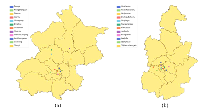
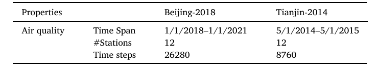
实验中使用的两个数据集分别来自北京和天津的空气质量监测站。两个城市的站点具有相同的采集时间间隔，即每小时一次，但采集的数据集来自不同的时期。

1. Beijing-2018，其中包含从2018年1月1日到2021年1月1日的 PM2.5数据，共计26280个时间步长。它包括12个选定的监测站。
   2.Tianjin-2014，其中包含从2014年5月1日到2015年5月1日共8760个时间步长的PM2.5数据。它包括12个选定的监测站。
   
   
   数据预处理：使用 PauTa 准则检测并删除数据集中出现的异常值。然后使用线性插值补充缺失值和错误值。此外，还使用ZScore方法对数据进行归一化，以促进模型收敛。将预处理后的数据集以8:1:1的比例分为训练集、验证集和测试集。

（2）评估标准
MAE:

RMSE:

论文以ARIMA、LSTM、TCN、CNN-LSTM、Reformer、Informer、STGCN作为基线对比所提出的方法的实验效果。
（3）实验结果
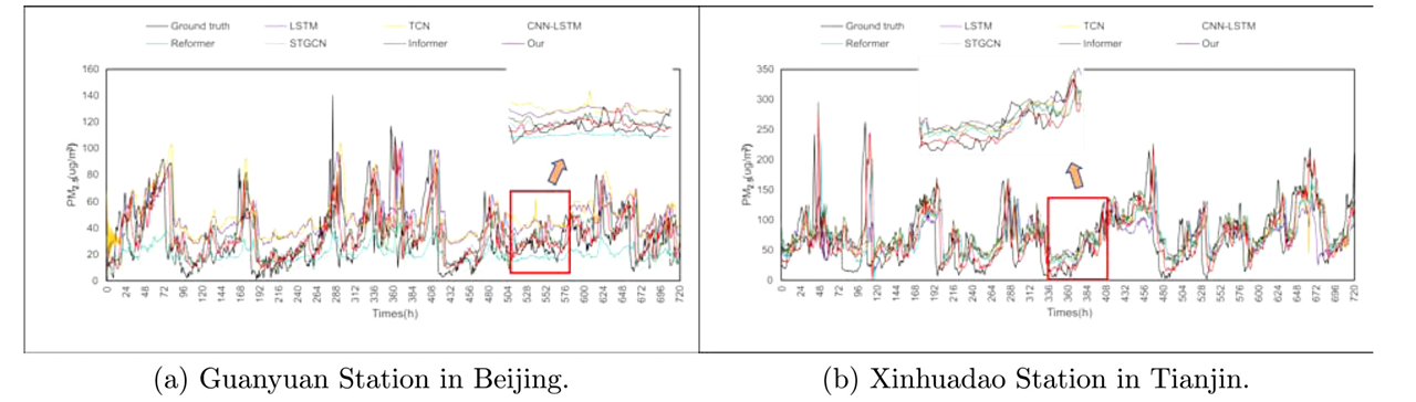
为评估模型在短期预测的性能，作者首先进行了单步实验分析，实验结果如下图所示：

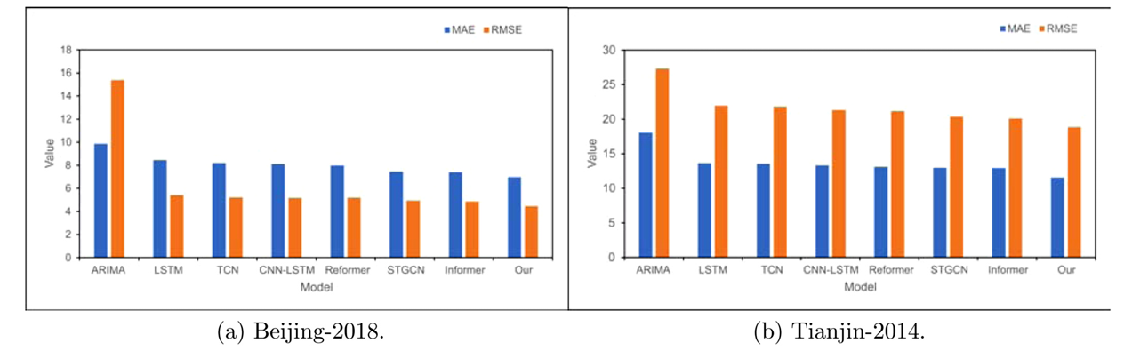
由上述实验结果可知，与短期预测任务中的基线相比，所提出的模型表现出卓越的性能。LSTM、TCN和其他模型的预测结果优于传统的统计模型ARIMA，这表明深度学习方法可以有效地模拟非线性时i相关性。CNN-LSTM和STGCN优于LSTM和TCN，这表明捕获时空相关性优于单独捕获时间相关性。与STGCN相比，所提出的模型显示出更好的性能，表明使用多个图可以更全面地表示信息。
评估模型在长期预测的鲁棒性，作者进行了多步预测实验，实验结果如下：


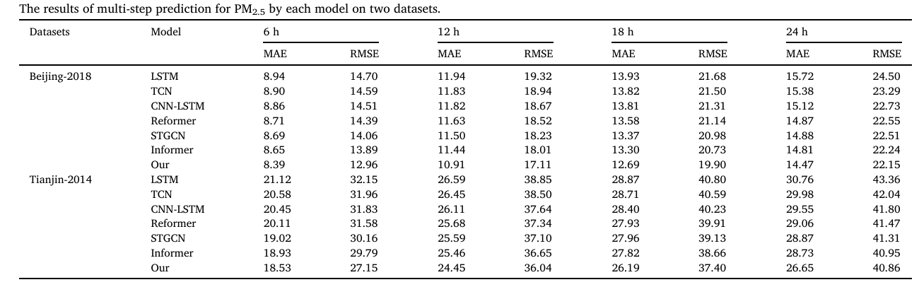
上述表格显示了每个模型的多步骤PMprediction的结果。可以观察到，所有模型的MAE 和RMSE值都随着预测时间步长的增加而增加。折线图为两个数据集在一个月内预测的PM浓度（预测范围为9 h)的可视化。从图中可以观察到，与其他模型相比，所提出的模型表现出MAE和RMSE的最小值，表明其在多步预测方面具有优势。
（4）消融研究
为了评估整个组件中多图结构中两个新构建的图的性能，作者进行了消融研究。作者将没有邻居图和没有时序因果图的模型与多图模型进行实验比较，实验结果如下：

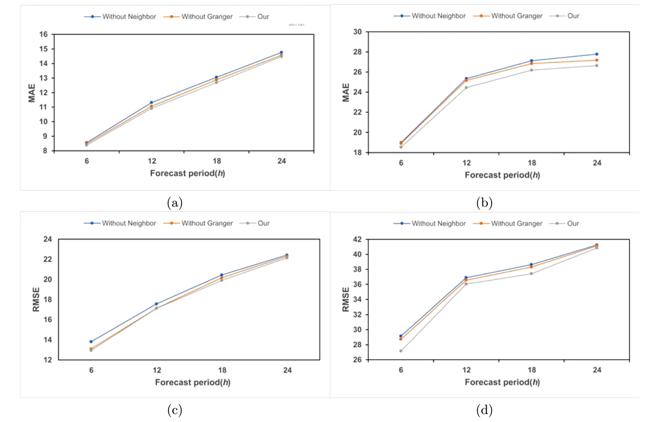
通过比较可以发现，随着预测步骤的扩展，两个变体和整个多重图模型的预测误差也会增加。相比之下，完整的多图模型在每个时间步长的预测误差最小。这表明构建的多图模型确实可以提高预测精度，尤其是在短期预测中。此外，，没有时间因果关系图的变体的预测误差是三者中最大的。这表明构建的时间因果关系图确实有助于提高预测准确性。
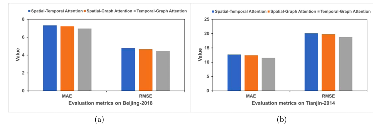
(5)注意力性能研究
为评估时空多图注意力机制的性能，作者进行了该部分的实验研究，将其在单步和多步预测中的结果与时间-空间注意力机制和空间图注意力机制的结果进行了比较，单步预测实验结果如下所示：

多步预测实验结果如下：

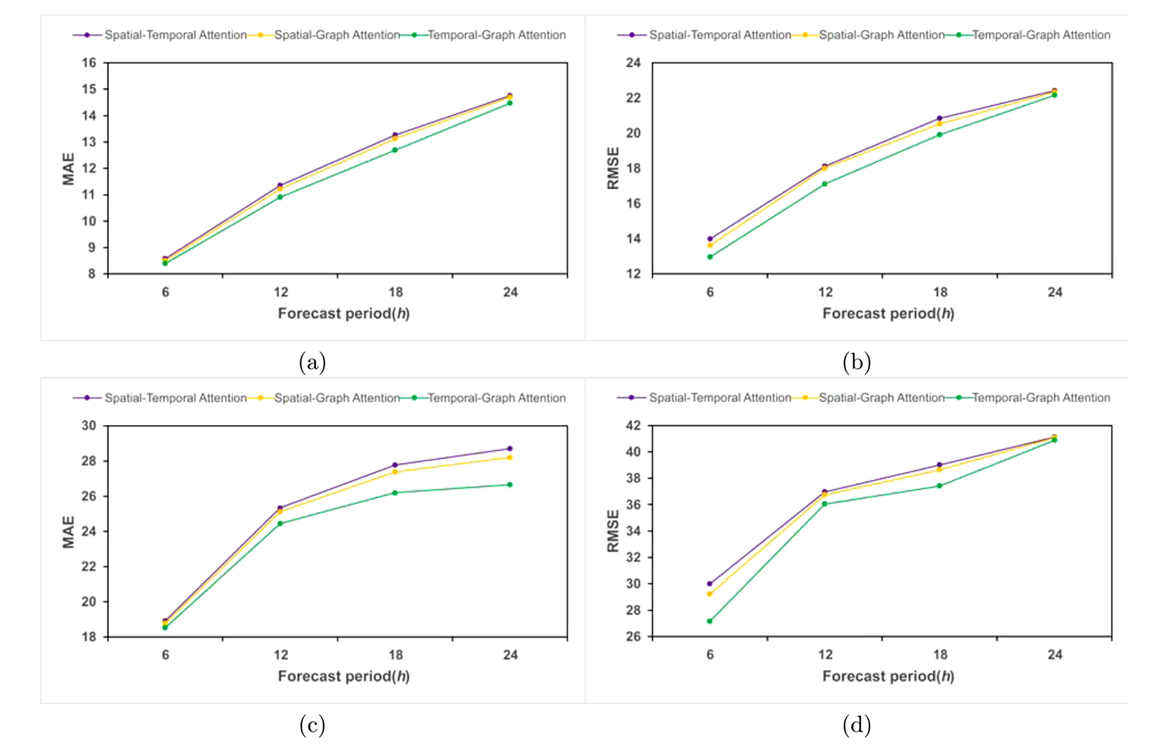
由结果可知，无论是单步还是多步预测，论文提出的模型都得到了最好的预测结果。这表明所提出的时间图注意力机制在时空多图预测中具有优势。

总结

在过去的学习当中，大部分学习的文献都是水质预测方面的，没有怎么看过大气预测方向的论文，后续我会花时间看这方面的论文。通过本周的学习我对多图构建有了一定的了解，在后续，可以考虑利用这一输入的构建的方法从而增加论文的新颖性。