当前位置：首页 > news >正文

脚本更新--CosMx、Xenium的neighborhood analysis（R版本）

news 2025/10/25 8:37:14

作者，Evil Genius

今天我们更新脚本

实现的方法

我们实现任何的分析内容，都建立在基础扎实的情况下，基础内容一定要引起大家的重视，不然上这些针对课题的个性化分析会非常吃力，还是建议大家参加一下2025番外--linux、R、python培训https://mp.weixin.qq.com/s?__biz=Mzg2MDY1NTYyOQ==&mid=2247498483&idx=1&sn=e75514e7725daec3dca32370d665119c&scene=21#wechat_redirect我们来用R实现

library(Seurat)
library(tidyverse)
library(dplyr)
library(ggplot2)Lymphoma_data <- readRDS("Lymphoma_data.rds")

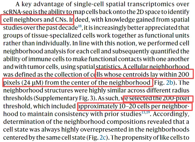
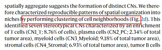
neighborhood analysis,现在都是拼片的，分析就是统计每个细胞周围细胞的种类和数量。

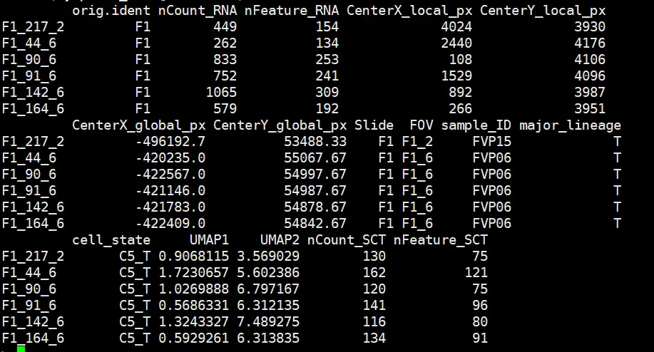
Lymphoma.meta <- Lymphoma_data@meta.data
major.ord = unique(Lymphoma.meta$cell_state)
my_neighbor_list <- list()
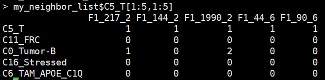
for (clstype in major.ord){my.neighbor = c()print (clstype)for(sam in unique(Lymphoma.meta$FOV)) {print (sam)tmp.meta = Lymphoma.meta[Lymphoma.meta$cell_state == clstype & Lymphoma.meta$FOV == sam, ]tmp.meta1 = Lymphoma.meta[Lymphoma.meta$FOV == sam, ]if(clstype %in% unique(tmp.meta1$cell_state)){tmp.mtx = matrix(0,nrow = length(major.ord),ncol = nrow(tmp.meta))rownames(tmp.mtx) = major.ordcolnames(tmp.mtx) = rownames(tmp.meta)for(i in 1:nrow(tmp.meta)) {xloc = tmp.meta[i, 'CenterX_local_px']yloc = tmp.meta[i, 'CenterY_local_px']cutoff = 200idx1 = tmp.meta1[, 'CenterX_local_px'] <=  (xloc + cutoff) & tmp.meta1[,'CenterX_local_px'] >=  (xloc - cutoff)idx2 = tmp.meta1[, 'CenterY_local_px'] <=  (yloc + cutoff) & tmp.meta1[,'CenterY_local_px'] >=  (yloc - cutoff)square = tmp.meta1[idx1 & idx2,]dis = apply(square, 1, function(x) {sqrt((as.numeric(x['CenterX_local_px']) - as.numeric(xloc))^2 + (as.numeric(x['CenterY_local_px']) - as.numeric(yloc))^2)} )tmp.freq = table(tmp.meta1[match(names(dis[dis <= cutoff]), rownames(tmp.meta1)), 'cell_state'])tmp.mtx[,i] = tmp.freq[match(major.ord,names(tmp.freq))]}tmp.mtx[which(is.na(tmp.mtx))] = 0my.neighbor = cbind(my.neighbor, tmp.mtx)}}my_neighbor_list[[clstype]] <- my.neighborwrite.csv(t(my.neighbor), paste0('./neighborhood/',clstype,'.neighbor.sub.csv'),quote = F)
}

merge neighborhood composition count matrix for all cells

cell_neighbor_df <- c()
for(i in 1:length(my_neighbor_list)){df <- as.data.frame(t(my_neighbor_list[[i]]))df$center_cell_state <- names(my_neighbor_list)[i]cell_neighbor_df <- rbind(cell_neighbor_df, df)
}# aggregrate neighborhood cell counts by center cell type #
cell_state <- unique(Lymphoma.meta$cell_state)
Neighbor_sum <- matrix(0, nrow=19, ncol=19)
rownames(Neighbor_sum) = cell_state
colnames(Neighbor_sum) = cell_statefor(i in cell_state){df_filter <- filter(cell_neighbor_df, cell_neighbor_df$center_cell_state == i)df_filter <- df_filter[,cell_state]df_filter_sum = colSums(df_filter)Neighbor_sum[i,] = df_filter_sum
}Neighbor_sum <- as.data.frame(Neighbor_sum)
Neighbor_sum$center_cell_state <- rownames(Neighbor_sum)# calculate cell proportion in each type of neighborhoods #
cell.prop <- as.data.frame(prop.table(as.matrix(Neighbor_sum[,0:19]), margin=1))
cell.prop$center_cell_state <- rownames(cell.prop)cell.prop <- reshape2::melt(cell.prop, id.vars=c("center_cell_state"),measure.vars= cell_state,variable.name = "neighbor_cell_state", value.name="neighbor_cell_prop")cell.prop$center_cell_state <- factor(cell.prop$center_cell_state, levels=c("C0_Tumor-B","C1_PC_IgG","C2_PC_IgA","C3_Resting-B","C4_PC_IgM","C5_T","C6_TAM_APOE_C1Q","C7_TAM_SPP1","C8_Mac_DUSP1","C9_Mac_CXCL8","C10_Mac_MT2A","C11_FRC","C12_HEV","C13_Endothelial_VWF","C14_VSMC","C15_Stromal_CLU","C16_Stressed","C17_Epithelial","C18_RBC"))              
cell.prop$neighbor_cell_state <- factor(cell.prop$neighbor_cell_state, levels=c("C0_Tumor-B","C1_PC_IgG","C2_PC_IgA","C3_Resting-B","C4_PC_IgM","C5_T","C6_TAM_APOE_C1Q","C7_TAM_SPP1","C8_Mac_DUSP1","C9_Mac_CXCL8","C10_Mac_MT2A","C11_FRC","C12_HEV","C13_Endothelial_VWF","C14_VSMC","C15_Stromal_CLU","C16_Stressed","C17_Epithelial","C18_RBC"))              # plot #
ggplot(cell.prop,aes(center_cell_state, neighbor_cell_prop, fill=neighbor_cell_state))+geom_bar(stat = "identity",position = "fill")+ggtitle("Neighboring cell proportion for each cell state")+theme_classic()+theme(axis.ticks.length = unit(0.5,'cm'))+theme(axis.text.x = element_text(angle=60,hjust = 1))+guides(fill=guide_legend(title = "Cell type"))+scale_fill_manual(values = c("#96F148","#ff7f00","#e5f5f9","#bebada","#df65b0","#D10000","#0000FF","#fff7fb","#fccde5","#bc80bd","#d9d9d9","#ffed6f","#d6604d","#02818a","#ccecb5","#80b1d3","#fb9a99","#006837","#6a3d9a"))

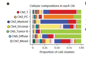
CN聚类分析

cell_neighbor_pca <- prcomp(cell_neighbor_df[,1:19])
cell_neighbor_pca_coord <- as.data.frame(cell_neighbor_pca$x)
cell_neighbor_pca_coord <- rownames_to_column(cell_neighbor_pca_coord, var="Barcode")
cell_neighbor_pca_coord <- left_join(cell_neighbor_pca_coord, spatial_niche, by="Barcode")library(plotly)
plot_ly(cell_neighbor_pca_coord, x = ~PC1, y = ~PC2, z = ~PC3, color = ~CN_cluster,colors=c("#ed2224","#fbb14d","#3B50A3","#eee817","#79c479","#55C7F3","#dad9d9"),alpha=0.7, sizes= c(50,50))# plot cell composition in each CN (Figure 2e) #
Lymphoma.meta <- rownames_to_column(Lymphoma.meta, var="Barcode")
Lymphoma.meta <- left_join(Lymphoma.meta, spatial_niche, by="Barcode")cellnum <- table(Lymphoma.meta$cell_state, Lymphoma.meta$CN_cluster)
cellnum
cell.prop <- as.data.frame(prop.table(cellnum))
colnames(cell.prop)<-c("cell_state","CN_cluster","Proportion")
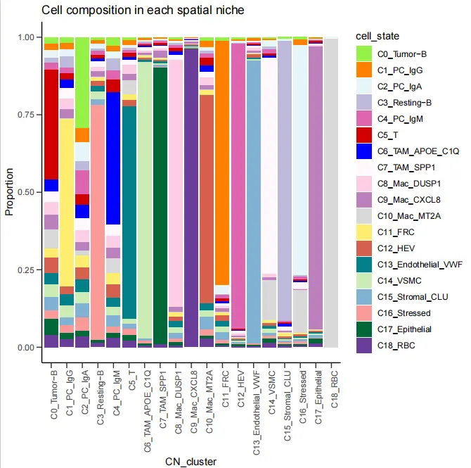
cell.prop$cell_state <- factor(cell.prop$cell_state, levels=c("C0_Tumor-B","C1_PC_IgG","C2_PC_IgA","C3_Resting-B","C4_PC_IgM","C5_T","C6_TAM_APOE_C1Q","C7_TAM_SPP1","C8_Mac_DUSP1","C9_Mac_CXCL8","C10_Mac_MT2A","C11_FRC","C12_HEV","C13_Endothelial_VWF","C14_VSMC","C15_Stromal_CLU","C16_Stressed","C17_Epithelial","C18_RBC"))ggplot(cell.prop,aes(CN_cluster,Proportion,fill=cell_state))+geom_bar(stat = "identity",position = "fill")+ggtitle("Cell composition in each spatial niche")+theme_bw()+scale_fill_manual(values=c("#96F148","#ff7f00","#e5f5f9","#bebada","#df65b0","#D10000","#0000FF","#fff7fb","#fccde5","#bc80bd","#d9d9d9","#ffed6f","#d6604d","#02818a","#ccecb5","#80b1d3","#fb9a99","#006837","#6a3d9a"))+theme_classic()+theme(axis.ticks.length = unit(0.2,'cm'))+ theme(axis.text.x = element_text(angle = 90,hjust = 1))guides(fill=guide_legend(title = NULL))