当前位置：首页 > news >正文

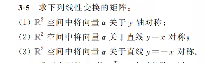
求下列线性变换的矩阵

news 2025/10/24 9:19:16

在这里插入图片描述

线性变换的矩阵表示

背景知识

在线性代数中，线性变换是指满足以下两个条件的变换 $\mathbb{R}^n \to \mathbb{R}^m$ ：

$T (u + v) = T (u) + T (v)$ （可加性）
$T (c u) = c T (u)$ （齐次性）

对于任意向量 $\in \mathbb{R}^n$ 和标量 $\in \mathbb{R}$ 。

线性变换的矩阵表示：给定线性变换 $\mathbb{R}^n \to \mathbb{R}^n$ 和标准基 ${e_1, e_2, ..., e_n\}$ ，变换 $T$ 对应的矩阵 $A$ 的第 $i$ 列就是 $T(e_i)$ 在标准基下的坐标表示。

在 $R2\mathbb{R}^2$ 中，标准基为：
$e1=(10),e2=(01)e_1 = \begin{pmatrix} 1 \\ 0 \end{pmatrix}, \quad e_2 = \begin{pmatrix} 0 \\ 1 \end{pmatrix}$

线性变换的矩阵表示基本原理

线性变换的矩阵表示基于一个核心思想：矩阵的列就是标准基向量经过变换后的坐标。

标准基的重要性

在 $Rn\mathbb{R}^n$ 中，标准基向量为：
$e1=(10⋮0),e2=(01⋮0),…,en=(00⋮1)e_1 = \begin{pmatrix} 1 \\ 0 \\ \vdots \\ 0 \end{pmatrix}, \quad e_2 = \begin{pmatrix} 0 \\ 1 \\ \vdots \\ 0 \end{pmatrix}, \quad \ldots, \quad e_n = \begin{pmatrix} 0 \\ 0 \\ \vdots \\ 1 \end{pmatrix}$

这些基向量的重要性在于：

任何向量 $\begin{pmatrix} x_1 \\ x_2 \\ \vdots \\ x_n \end{pmatrix}$ 都可以表示为 $x_1e_1 + x_2e_2 + \cdots + x_ne_n$
如果我们知道每个基向量 $e_i$ 经过变换 $T$ 后的结果，就能确定任意向量 $v$ 的变换结果

矩阵-向量乘法的列视角

考虑矩阵 $A$ 与向量 $x$ 的乘法：
$\begin{pmatrix} a_{11} & a_{12} & \cdots & a_{1n} \\ a_{21} & a_{22} & \cdots & a_{2n} \\ \vdots & \vdots & \ddots & \vdots \\ a_{n1} & a_{n2} & \cdots & a_{nn} \end{pmatrix} \begin{pmatrix} x_1 \\ x_2 \\ \vdots \\ x_n \end{pmatrix} = x_1\begin{pmatrix} a_{11} \\ a_{21} \\ \vdots \\ a_{n1} \end{pmatrix} + x_2\begin{pmatrix} a_{12} \\ a_{22} \\ \vdots \\ a_{n2} \end{pmatrix} + \cdots + x_n\begin{pmatrix} a_{1n} \\ a_{2n} \\ \vdots \\ a_{nn} \end{pmatrix}$

这个公式表明：

矩阵 $A$ 的第 $i$ 列就是 $Ae_i$ 的结果
矩阵-向量乘法实际上是输入向量各分量与矩阵各列的线性组合

题目求解

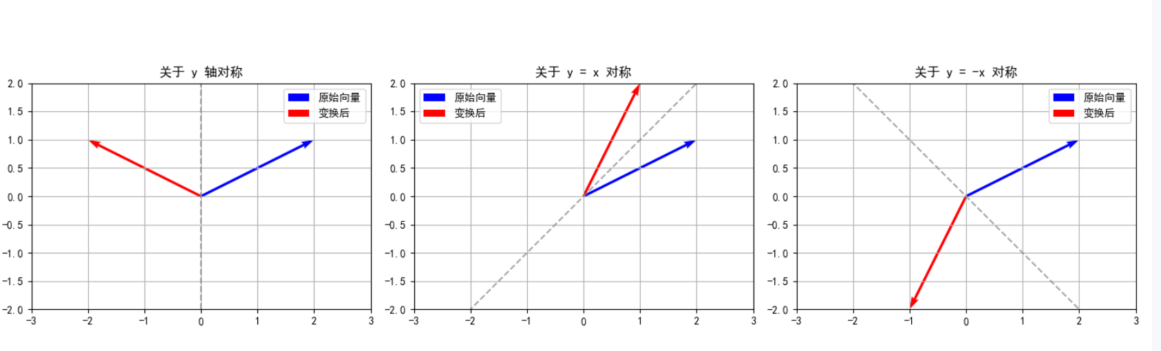
(1) 关于 $y$ 轴对称

变换规则： $\mapsto (-x, y)$

计算标准基的变换：

$T(e1)=T(10)=(−10)=−1⋅e1+0⋅e2T(e_1) = T\begin{pmatrix} 1 \\ 0 \end{pmatrix} = \begin{pmatrix} -1 \\ 0 \end{pmatrix} = -1 \cdot e_1 + 0 \cdot e_2$
$T(e2)=T(01)=(01)=0⋅e1+1⋅e2T(e_2) = T\begin{pmatrix} 0 \\ 1 \end{pmatrix} = \begin{pmatrix} 0 \\ 1 \end{pmatrix} = 0 \cdot e_1 + 1 \cdot e_2$

矩阵表示：
$A1=(−1001)A_1 = \begin{pmatrix} -1 & 0 \\ 0 & 1 \end{pmatrix}$

验证：
$(−1001)(xy)=(−xy)\begin{pmatrix} -1 & 0 \\ 0 & 1 \end{pmatrix} \begin{pmatrix} x \\ y \end{pmatrix} = \begin{pmatrix} -x \\ y \end{pmatrix}$

(2) 关于直线 $y = x$ 对称

变换规则： $\mapsto (y, x)$

计算标准基的变换：

$T(e1)=T(10)=(01)=0⋅e1+1⋅e2T(e_1) = T\begin{pmatrix} 1 \\ 0 \end{pmatrix} = \begin{pmatrix} 0 \\ 1 \end{pmatrix} = 0 \cdot e_1 + 1 \cdot e_2$
$T(e2)=T(01)=(10)=1⋅e1+0⋅e2T(e_2) = T\begin{pmatrix} 0 \\ 1 \end{pmatrix} = \begin{pmatrix} 1 \\ 0 \end{pmatrix} = 1 \cdot e_1 + 0 \cdot e_2$

矩阵表示：
$A2=(0110)A_2 = \begin{pmatrix} 0 & 1 \\ 1 & 0 \end{pmatrix}$

验证：
$(0110)(xy)=(yx)\begin{pmatrix} 0 & 1 \\ 1 & 0 \end{pmatrix} \begin{pmatrix} x \\ y \end{pmatrix} = \begin{pmatrix} y \\ x \end{pmatrix}$

(3) 关于直线 $y = - x$ 对称

变换规则： $\mapsto (-y, -x)$

计算标准基的变换：

$T(e1)=T(10)=(0−1)=0⋅e1−1⋅e2T(e_1) = T\begin{pmatrix} 1 \\ 0 \end{pmatrix} = \begin{pmatrix} 0 \\ -1 \end{pmatrix} = 0 \cdot e_1 - 1 \cdot e_2$
$T(e2)=T(01)=(−10)=−1⋅e1+0⋅e2T(e_2) = T\begin{pmatrix} 0 \\ 1 \end{pmatrix} = \begin{pmatrix} -1 \\ 0 \end{pmatrix} = -1 \cdot e_1 + 0 \cdot e_2$

矩阵表示：
$A3=(0−1−10)A_3 = \begin{pmatrix} 0 & -1 \\ -1 & 0 \end{pmatrix}$

验证：
$(0−1−10)(xy)=(−y−x)\begin{pmatrix} 0 & -1 \\ -1 & 0 \end{pmatrix} \begin{pmatrix} x \\ y \end{pmatrix} = \begin{pmatrix} -y \\ -x \end{pmatrix}$

图表

变换类型	矩阵表示
关于 $y$ 轴对称	$(−1001)\begin{pmatrix} -1 & 0 \\ 0 & 1 \end{pmatrix}$
关于 $y = x$ 对称	$(0110)\begin{pmatrix} 0 & 1 \\ 1 & 0 \end{pmatrix}$
关于 $y = - x$ 对称	$(0−1−10)\begin{pmatrix} 0 & -1 \\ -1 & 0 \end{pmatrix}$

运行代码可视化

python代码

import numpy as np
import matplotlib.pyplot as plt
# 设置中文字体
plt.rcParams['font.sans-serif'] = ['SimHei']  # 解决中文显示问题-设置字体为黑体
plt.rcParams['axes.unicode_minus'] = False  # 解决保存图像是负号'-'显示为方块的问题# 定义标准基向量
e1 = np.array([1, 0])
e2 = np.array([0, 1])print("标准基向量:")
print(f"e1 = {e1}")
print(f"e2 = {e2}")
print()# (1) 关于 y 轴对称的变换
def reflection_y(vec):"""关于 y 轴对称变换"""return np.array([-vec[0], vec[1]])# 计算标准基的变换结果
T_e1_y = reflection_y(e1)
T_e2_y = reflection_y(e2)# 构建变换矩阵
A_y = np.column_stack([T_e1_y, T_e2_y])
print("(1) 关于 y 轴对称的变换矩阵:")
print(A_y)# (2) 关于直线 y = x 对称的变换
def reflection_y_eq_x(vec):"""关于直线 y = x 对称变换"""return np.array([vec[1], vec[0]])# 计算标准基的变换结果
T_e1_yx = reflection_y_eq_x(e1)
T_e2_yx = reflection_y_eq_x(e2)# 构建变换矩阵
A_yx = np.column_stack([T_e1_yx, T_e2_yx])
print("(2) 关于直线 y = x 对称的变换矩阵:")
print(A_yx)# (3) 关于直线 y = -x 对称的变换
def reflection_y_eq_minus_x(vec):"""关于直线 y = -x 对称变换"""return np.array([-vec[1], -vec[0]])# 计算标准基的变换结果
T_e1_ymx = reflection_y_eq_minus_x(e1)
T_e2_ymx = reflection_y_eq_minus_x(e2)# 构建变换矩阵
A_ymx = np.column_stack([T_e1_ymx, T_e2_ymx])
print("(3) 关于直线 y = -x 对称的变换矩阵:")
print(A_ymx)# 可视化变换结果
def plot_transformations():"""绘制变换效果图"""fig, axes = plt.subplots(1, 3, figsize=(15, 5))# 原始向量original = np.array([2, 1])# (1) 关于 y 轴对称axes[0].quiver(0, 0, original[0], original[1], angles='xy', scale_units='xy', scale=1, color='blue',label='原始向量')transformed = A_y @ originalaxes[0].quiver(0, 0, transformed[0], transformed[1], angles='xy', scale_units='xy', scale=1, color='red',label='变换后')axes[0].axvline(x=0, color='gray', linestyle='--', alpha=0.7)axes[0].set_xlim(-3, 3)axes[0].set_ylim(-2, 2)axes[0].set_aspect('equal')axes[0].set_title('关于 y 轴对称')axes[0].legend()axes[0].grid(True)# (2) 关于直线 y = x 对称axes[1].quiver(0, 0, original[0], original[1], angles='xy', scale_units='xy', scale=1, color='blue',label='原始向量')transformed = A_yx @ originalaxes[1].quiver(0, 0, transformed[0], transformed[1], angles='xy', scale_units='xy', scale=1, color='red',label='变换后')x = np.linspace(-3, 3, 100)axes[1].plot(x, x, 'gray', linestyle='--', alpha=0.7)axes[1].set_xlim(-3, 3)axes[1].set_ylim(-2, 2)axes[1].set_aspect('equal')axes[1].set_title('关于 y = x 对称')axes[1].legend()axes[1].grid(True)# (3) 关于直线 y = -x 对称axes[2].quiver(0, 0, original[0], original[1], angles='xy', scale_units='xy', scale=1, color='blue',label='原始向量')transformed = A_ymx @ originalaxes[2].quiver(0, 0, transformed[0], transformed[1], angles='xy', scale_units='xy', scale=1, color='red',label='变换后')axes[2].plot(x, -x, 'gray', linestyle='--', alpha=0.7)axes[2].set_xlim(-3, 3)axes[2].set_ylim(-2, 2)axes[2].set_aspect('equal')axes[2].set_title('关于 y = -x 对称')axes[2].legend()axes[2].grid(True)plt.tight_layout()plt.show()# 执行可视化
plot_transformations()