当前位置：首页 > news >正文

「用Python来学微积分」问题，二维图形关于任意直线的对称变换

news 2025/10/23 8:25:54

掌握线性变换的核心思想，用代码实现复杂的几何对称

一、分步变换法

核心原理：化繁为简的变换策略

对称变换是计算机图形学的基础操作，但关于任意直线的对称听起来很复杂？其实秘诀在于：将复杂问题分解为简单步骤的组合。

关键步骤分解：

步骤	变换类型	目的与作用
1. 平移变换 (Translation)	平移	将直线的一点（如与Y轴交点或特定点）移动至坐标原点，使对称轴穿过原点。
2. 旋转变换 (Rotation)	旋转	将平移后的直线绕原点旋转，使其与X轴或Y轴重合，将问题简化为关于坐标轴的对称。
3. 核心对称变换 (Reflection)	对称（反射）	执行关于该坐标轴（如X轴）的对称变换，这是整个操作的核心镜像步骤。
4. 逆变换 (Inverse Transformations)	旋转逆变换 + 平移逆变换	将图形按相反顺序旋转和平移回原始位置，完成关于原始直线的最终对称。

下面我们使用 matplotlib和 numpy分步实现，每个步骤后都会绘制当前状态的图形

1. 导入必要的库

import numpy as np
import matplotlib.pyplot as plt
from matplotlib.patches import Polygon
import math# 设置中文字体
plt.rcParams['font.sans-serif'] = ['SimHei']
plt.rcParams['axes.unicode_minus'] = False

2. 定义初始图形和直线

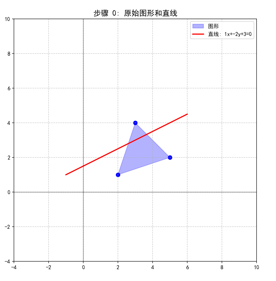
# 1. 定义原始图形（三角形）
original_vertices = np.array([[2, 1], [5, 2], [3, 4]])# 定义任意直线 Ax + By + C = 0
A, B, C = 1, -2, 3  # 直线 x - 2y + 3 = 0# 计算直线上的两个点用于绘图
if B != 0:x_line = np.array([-1, 6])y_line = (-A * x_line - C) / B
else:  # 处理垂直情况x_line = np.array([-C/A, -C/A])y_line = np.array([-1, 6])# 绘制初始状态
def plot_scene(vertices, line_points, title, step_num):fig, ax = plt.subplots(figsize=(8, 8))ax.set_aspect('equal')# 绘制图形polygon = Polygon(vertices, closed=True, fill=True, alpha=0.3, color='blue', label='图形')ax.add_patch(polygon)# 绘制顶点ax.scatter(vertices[:, 0], vertices[:, 1], color='blue', s=50)# 绘制直线ax.plot(line_points[0], line_points[1], 'r-', linewidth=2, label=f'直线: {A}x+{B}y+{C}=0')# 设置坐标轴ax.set_xlim(-2, 8)ax.set_ylim(-2, 8)ax.grid(True, linestyle='--', alpha=0.7)ax.axhline(y=0, color='k', linestyle='-', alpha=0.3)ax.axvline(x=0, color='k', linestyle='-', alpha=0.3)ax.set_title(f'步骤 {step_num}: {title}', fontsize=14)ax.legend()plt.show()# 绘制初始图形和直线
plot_scene(original_vertices, [x_line, y_line], "原始图形和直线", 0)

运行结果:

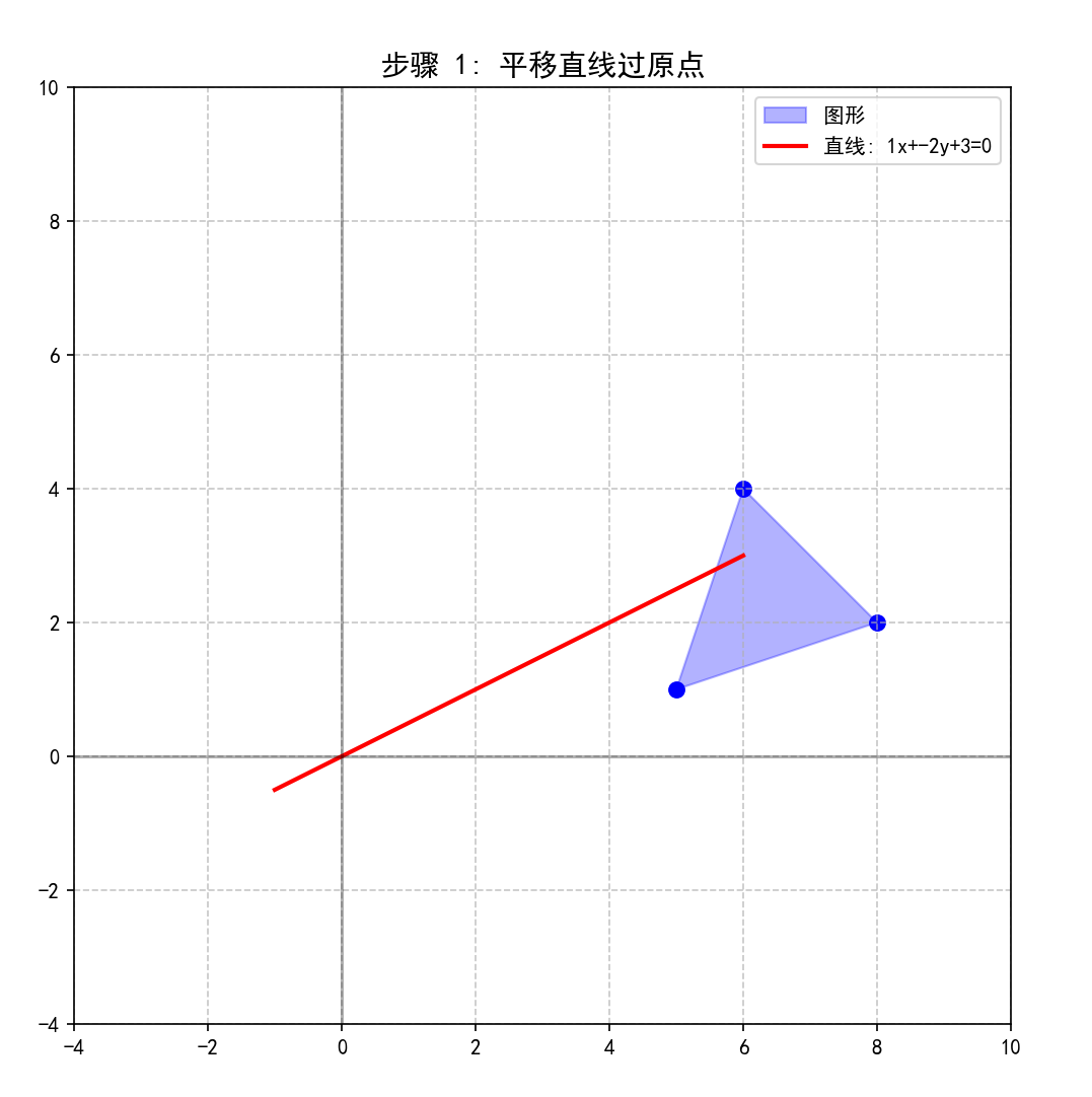
3. 步骤1：平移直线使其通过原点

目标是将直线的任意一点平移至坐标原点，从而使直线方程中的常数项 C 变为0。

操作：计算平移向量。通常可以选择直线的一个特定点，例如与X轴的交点 (-C/A, 0)或与Y轴的交点 (0, -C/B)，或者利用直线上已知的一点。平移向量为 (-T_x, -T_y)，其中 (T_x, T_y)是所选点的坐标。

变换矩阵 T₁：

    [ 1, 0, -T_x ][ 0, 1, -T_y ][0, 0, 1 ]

Python代码：

# 计算平移量：找到直线上一点，将其平移到原点
if A != 0:# 取直线与x轴交点translate_x = -C / Atranslate_y = 0
else:# 取直线与y轴交点translate_x = 0translate_y = -C / B
# 平移矩阵
translation_matrix = np.array([[1, 0, -translate_x],[0, 1, -translate_y],[0, 0, 1]])# 对图形顶点进行平移（齐次坐标）
def apply_transform(vertices, transform_matrix):homogeneous_coords = np.column_stack([vertices, np.ones(len(vertices))])transformed = homogeneous_coords @ transform_matrix.Treturn transformed[:, :2]# 应用平移变换
vertices_step1 = apply_transform(original_vertices, translation_matrix)# 更新直线方程（常数项C变为0）
C_step1 = A * (-translate_x) + B * (-translate_y) + C# 计算新直线上的点
if B != 0:y_line_step1 = (-A * x_line - C_step1) / B
else:y_line_step1 = y_line# 绘制步骤1结果
plot_scene(vertices_step1, [x_line, y_line_step1], "平移直线过原点", 1)

运行结果:

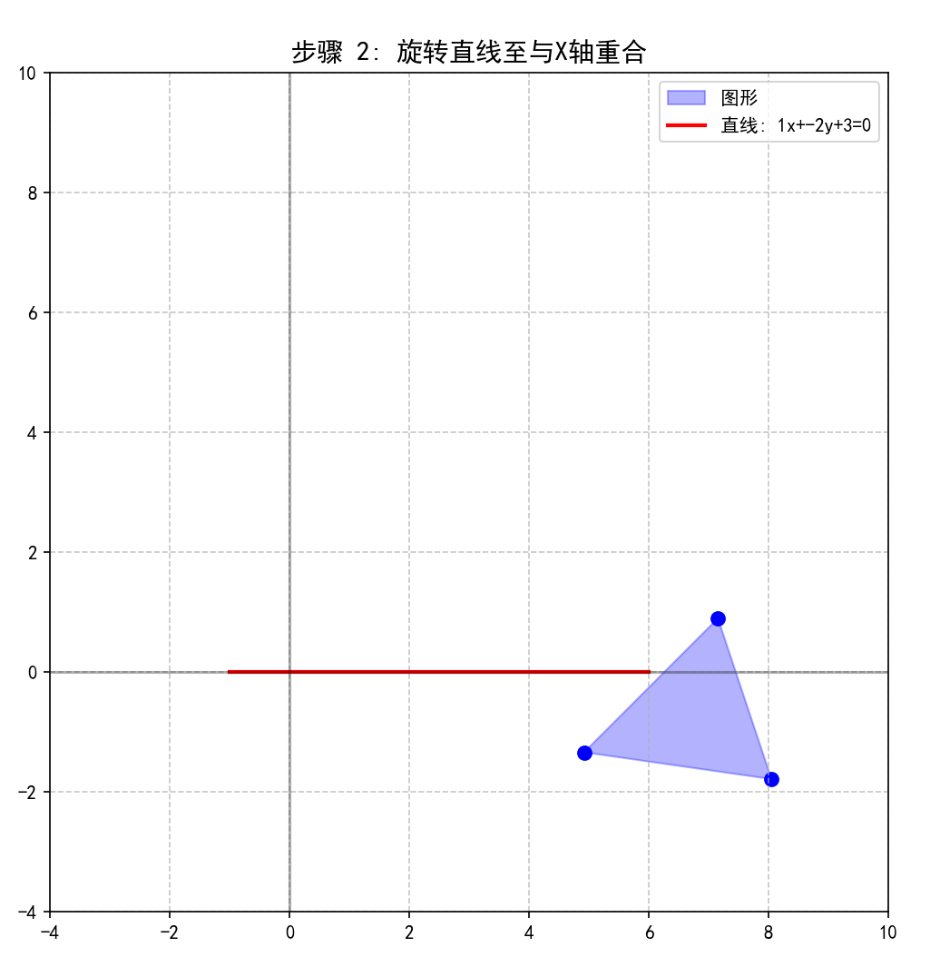
4. 步骤2：旋转直线使其与X轴重合

目标是将过原点的直线旋转到与X轴重合。

操作：计算旋转角度 θ。θ 是直线与X轴正方向的夹角。可以通过直线的方向向量或法向量求出。例如，直线法向量为 (A, B)，则其与X轴夹角 θ 满足 tan(θ) = B/A？实际上，旋转角应使得直线的法向量与Y轴平行。更准确地说，旋转角 θ 应满足 tan(θ) = -A/B（当B≠0时），因为直线的方向向量为 (B, -A)或 (-B, A)。为将直线旋转到X轴，需要旋转 -θ角度。

变换矩阵 R：

    [ cos(-θ), -sin(-θ), 0 ][ sin(-θ), cos(-θ),  0 ][    0,       0,     1 ]

Python代码:

# 计算直线与X轴的夹角
line_angle = math.atan2(A, -B)  # 法向量(A,B)与X轴夹角# 旋转矩阵（将直线旋转到X轴）
rotation_matrix = np.array([[math.cos(-line_angle), -math.sin(-line_angle), 0],[math.sin(-line_angle), math.cos(-line_angle), 0],[0, 0, 1]])# 应用旋转变换
vertices_step2 = apply_transform(vertices_step1, rotation_matrix)# 计算旋转后的直线（现在应与X轴重合）
# 直线方程变为：x = 0（在旋转后的坐标系中）
x_line_step2 = np.array([-1, 6])
y_line_step2 = np.array([0, 0])# 绘制步骤2结果
plot_scene(vertices_step2, [x_line_step2, y_line_step2], "旋转直线至与X轴重合", 2)

运行结果:

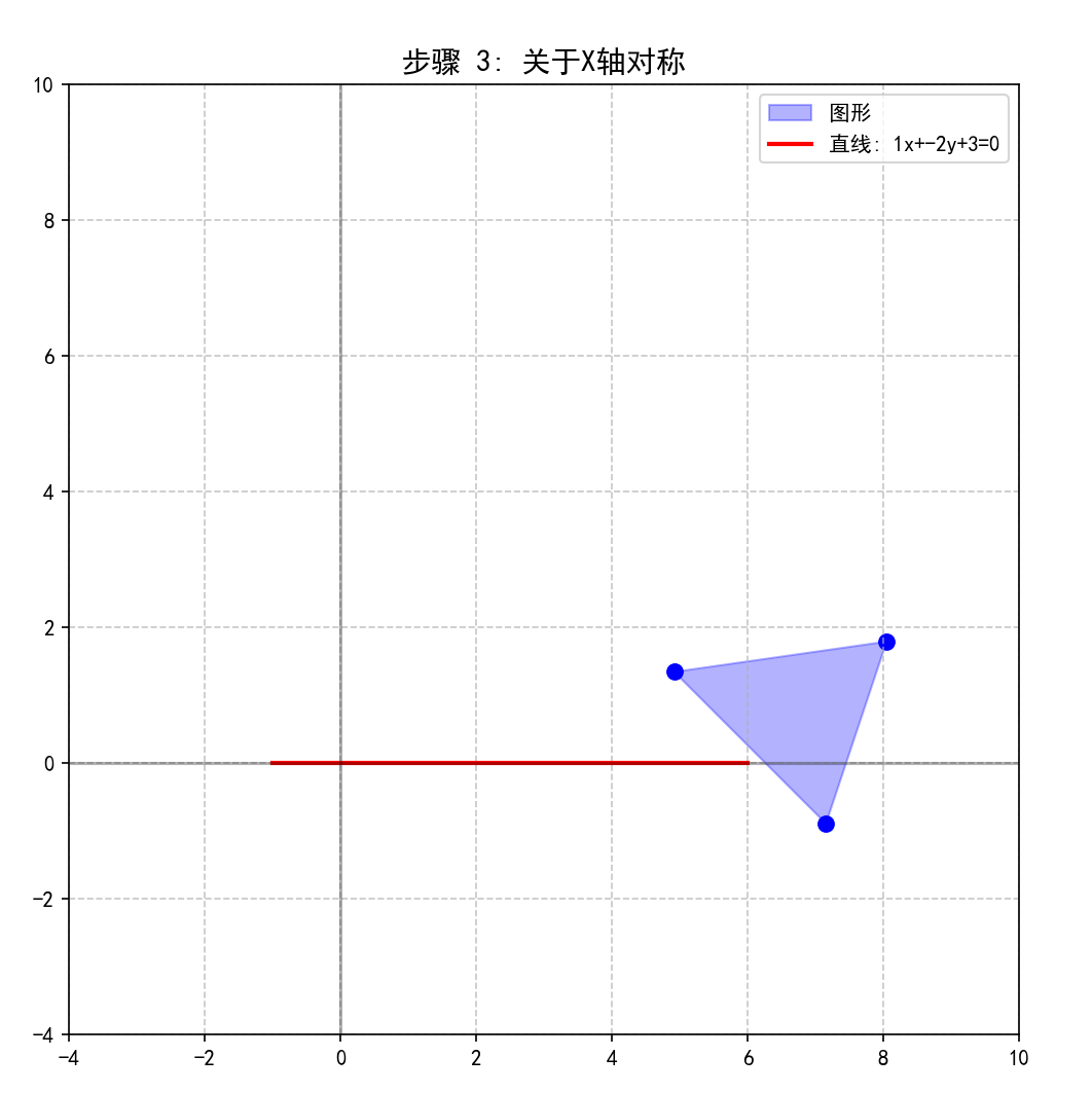
5. 步骤3：关于X轴对称变换

此时，图形已经位于一个“新坐标系”中，其中直线就是X轴。关于该直线的对称就简化为关于X轴的对称。

操作：将图形中所有点的Y坐标取反。
变换矩阵 M：

[ 1,  0, 0 ]
[ 0, -1, 0 ]
[ 0,  0, 1 ]

Python代码:

# 关于X轴对称的变换矩阵
reflection_matrix = np.array([[1, 0, 0],[0, -1, 0],[0, 0, 1]])# 应用对称变换
vertices_step3 = apply_transform(vertices_step2, reflection_matrix)# 直线保持不变（仍在X轴上）
x_line_step3 = x_line_step2
y_line_step3 = y_line_step2# 绘制步骤3结果
plot_scene(np.vstack([vertices_step2, vertices_step3]), [x_line_step3, y_line_step3], "关于X轴对称", 3)

运行结果:

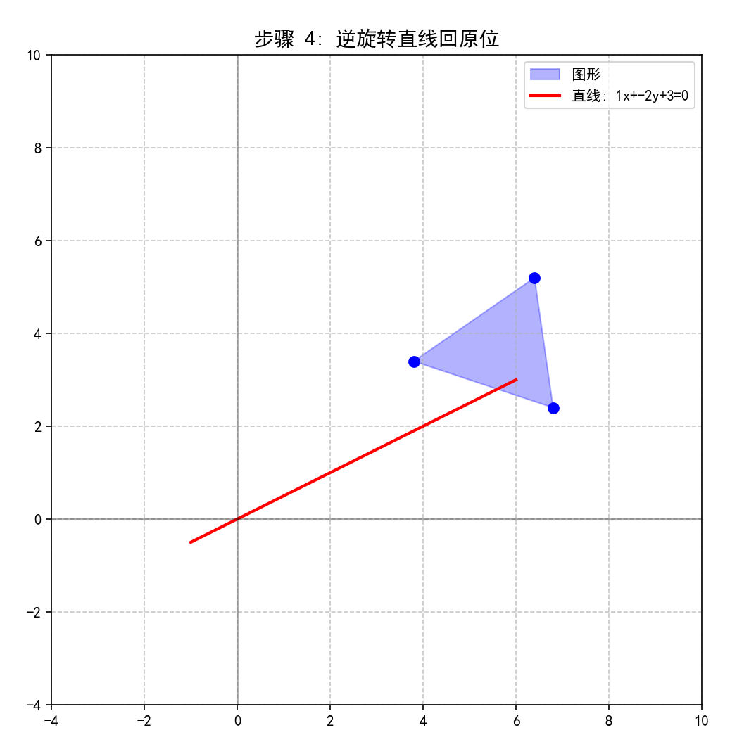
6. 步骤4: 逆旋转直线回原位

将坐标系旋转回第一步平移之后的状态。

操作：进行与第二步相反的旋转，角度为 -θ的逆运算，即旋转 θ角度。
变换矩阵 R⁻¹：

[ cosθ, -sinθ, 0 ]
[ sinθ,  cosθ, 0 ]
[  0,     0,   1 ]

Python代码:

# 逆旋转矩阵（转回原方向）
inverse_rotation_matrix = np.array([[math.cos(line_angle), -math.sin(line_angle), 0],[math.sin(line_angle), math.cos(line_angle), 0],[0, 0, 1]])# 应用逆旋转变换
vertices_step4 = apply_transform(vertices_step3, inverse_rotation_matrix)# 计算逆旋转后的直线
if B != 0:y_line_step4 = (-A * x_line - C_step1) / B
else:y_line_step4 = y_line# 绘制步骤4结果
plot_scene(vertices_step4, [x_line, y_line_step4], "逆旋转直线回原位", 4)

运行结果:

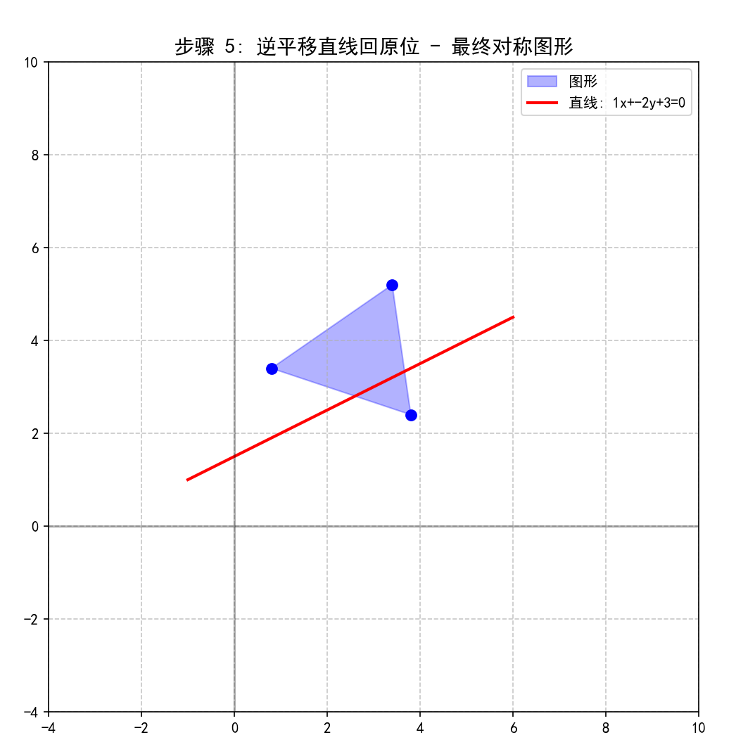
7. 步骤5: 逆平移直线回原位

将坐标系平移回原始位置。

操作：进行与第一步相反的平移。
变换矩阵 T₂：

[ 1, 0, 0 ]
[ 0, 1, 0 ]
[ T_x, T_y, 1 ]

Python代码:

# 逆平移矩阵
inverse_translation_matrix = np.array([[1, 0, translate_x],[0, 1, translate_y],[0, 0, 1]])# 应用逆平移变换
vertices_step5 = apply_transform(vertices_step4, inverse_translation_matrix)# 计算最终直线（回到原始位置）
if B != 0:y_line_final = (-A * x_line - C) / B
else:y_line_final = y_line# 绘制最终结果
plot_scene(vertices_step5, [x_line, y_line_final], "逆平移直线回原位 - 最终对称图形", 5)

运行结果:

二、直接用公式计算和可视化验证

1. 直接用公式计算

关于直线 Ax + By + C = 0 的对称点 (x', y') 的直接计算公式：

$\begin{align*} x' &= x - \frac{2A(Ax + By + C)}{A^2 + B^2} \\ y' &= y - \frac{2B(Ax + By + C)}{A^2 + B^2} \end{align*}$

Python代码:

import numpy as np
import matplotlib.pyplot as plt
from matplotlib.patches import Polygon
import math# 设置中文字体
plt.rcParams['font.sans-serif'] = ['SimHei']
plt.rcParams['axes.unicode_minus'] = Falsedef direct_line_symmetry(points, A, B, C):"""使用直接公式计算点关于直线的对称点公式: (x', y') = (x - 2A*(Ax+By+C)/(A²+B²), y - 2B*(Ax+By+C)/(A²+B²))"""points = np.array(points)denominator = A**2 + B**2if denominator < 1e-10:raise ValueError("直线方程系数A和B不能同时为零")symmetric_points = []for point in points:x, y = pointfactor = 2 * (A*x + B*y + C) / denominatorx_sym = x - A * factory_sym = y - B * factorsymmetric_points.append([x_sym, y_sym])return np.array(symmetric_points)

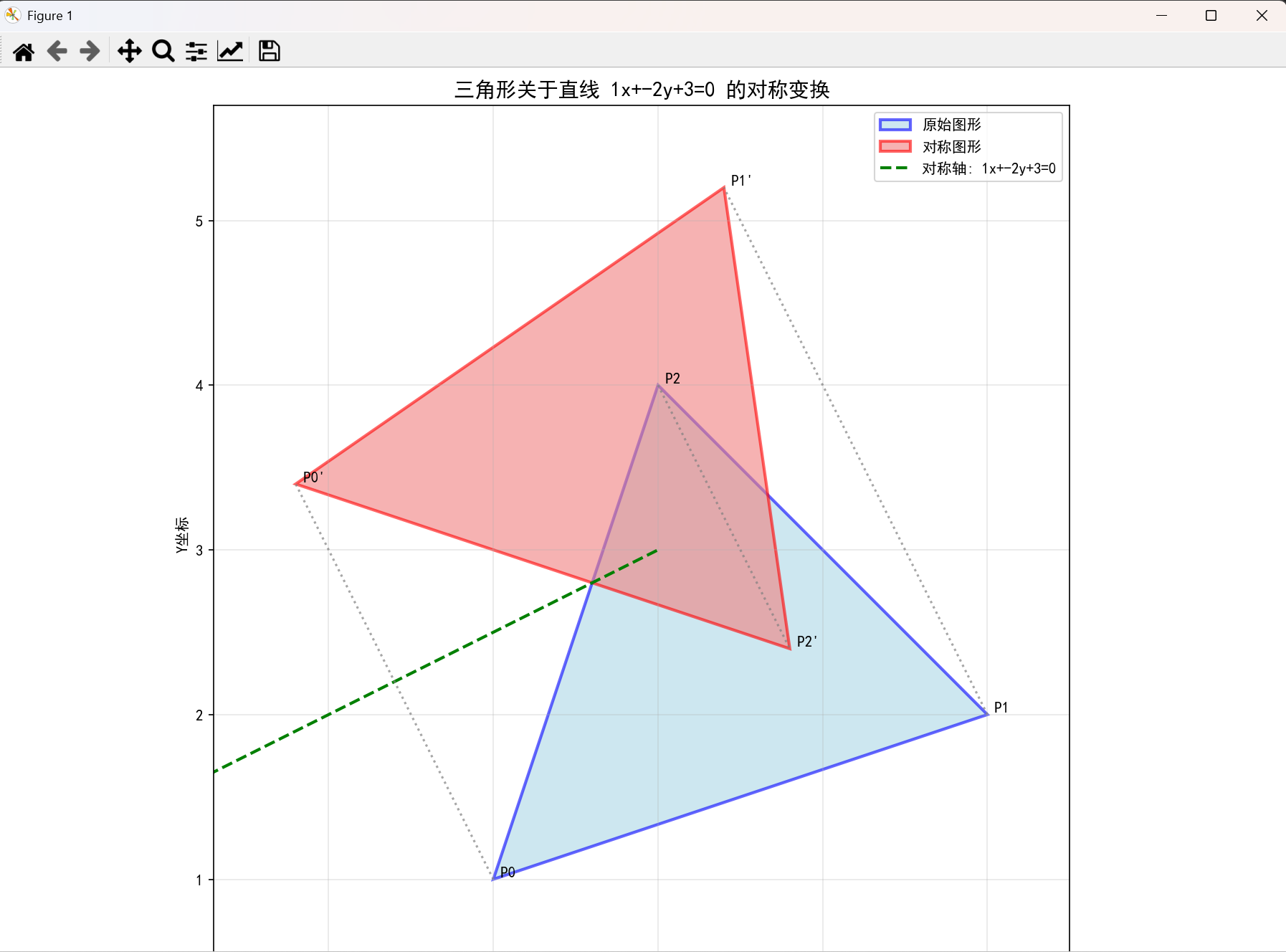
2. 添加可视化验证

def visualize_symmetry(points, A, B, C, title="二维图形关于直线的对称变换"):"""可视化原始图形和对称后的图形"""# 计算对称点symmetric_points = direct_line_symmetry(points, A, B, C)# 创建图形和坐标轴fig, ax = plt.subplots(1, 1, figsize=(12, 10))# 确保图形闭合original_closed = np.vstack([points, points[0]])symmetric_closed = np.vstack([symmetric_points, symmetric_points[0]])# 绘制原始图形（蓝色）original_polygon = Polygon(points, closed=True, alpha=0.6,facecolor='lightblue', edgecolor='blue', linewidth=2, label='原始图形')ax.add_patch(original_polygon)# 绘制对称图形（红色）symmetric_polygon = Polygon(symmetric_points, closed=True, alpha=0.6,facecolor='lightcoral', edgecolor='red', linewidth=2, label='对称图形')ax.add_patch(symmetric_polygon)# 绘制对称轴直线x_min, x_max = ax.get_xlim()y_min, y_max = ax.get_ylim()# 生成直线上的点if B != 0:x_line = np.array([x_min - 2, x_max + 2])  # 扩展范围确保直线可见y_line = (-A * x_line - C) / Belse:  # 垂直直线x_line = np.array([-C/A, -C/A])y_line = np.array([y_min - 2, y_max + 2])ax.plot(x_line, y_line, 'g--', linewidth=2, label=f'对称轴: {A}x+{B}y+{C}=0')# 绘制顶点连线，显示对称关系for i, (orig, sym) in enumerate(zip(points, symmetric_points)):ax.plot([orig[0], sym[0]], [orig[1], sym[1]], 'gray', linestyle=':', alpha=0.7)# 标记顶点编号ax.text(orig[0], orig[1], f' P{i}', fontsize=10, ha='left', va='bottom')ax.text(sym[0], sym[1], f" P{i}'", fontsize=10, ha='left', va='bottom')# 设置图形属性ax.set_xlabel('X坐标')ax.set_ylabel('Y坐标')ax.set_title(title, fontsize=14, fontweight='bold')ax.grid(True, alpha=0.3)ax.legend()ax.set_aspect('equal')# 自动调整坐标轴范围all_points = np.vstack([points, symmetric_points])margin = 0.5ax.set_xlim(all_points[:, 0].min() - margin, all_points[:, 0].max() + margin)ax.set_ylim(all_points[:, 1].min() - margin, all_points[:, 1].max() + margin)plt.tight_layout()plt.show()return symmetric_pointsdef compare_methods():"""测试并可视化对称变换"""# 测试点集（三角形）test_points = np.array([[2, 1], [5, 2], [3, 4]])A, B, C = 1, -2, 3  # 直线方程: x - 2y + 3 = 0print("原始顶点坐标:")for i, point in enumerate(test_points):print(f"P{i}: ({point[0]}, {point[1]})")result = direct_line_symmetry(test_points, A, B, C)print("\n对称后顶点坐标:")for i, point in enumerate(result):print(f"P{i}': ({point[0]:.2f}, {point[1]:.2f})")# 可视化symmetric_points = visualize_symmetry(test_points, A, B, C,f"三角形关于直线 {A}x+{B}y+{C}=0 的对称变换")return symmetric_points# 额外的示例：绘制不同图形的对称变换
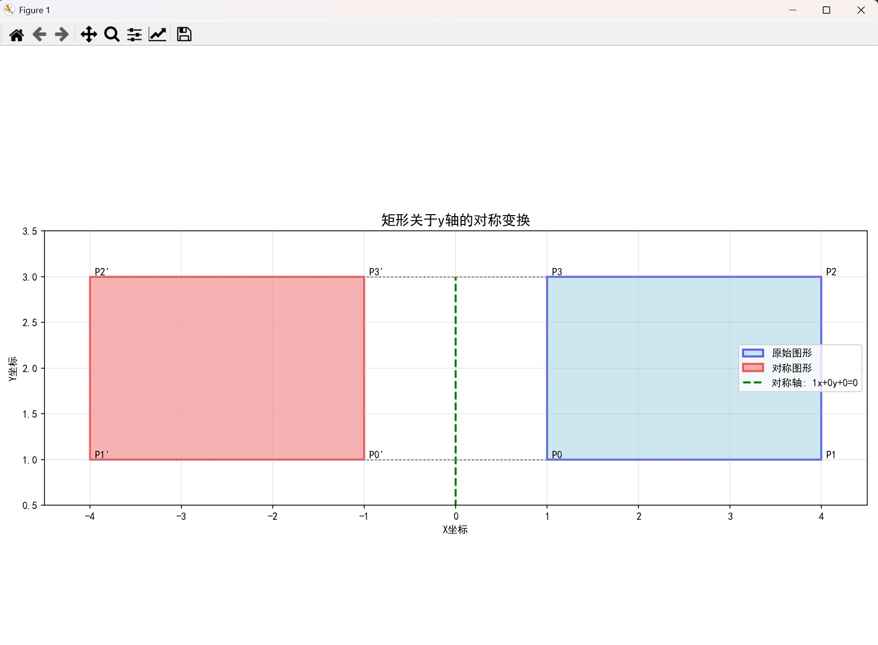
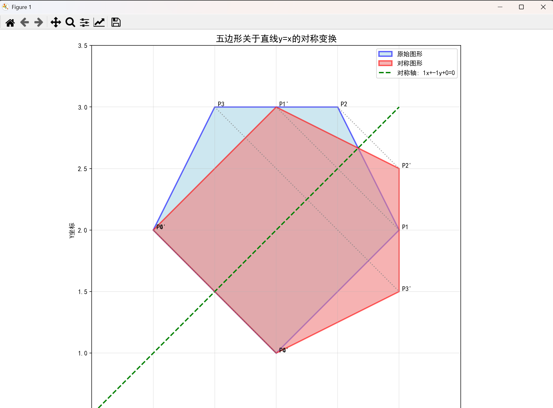
def additional_examples():"""更多对称变换示例"""# 示例1：矩形关于y轴对称rectangle_points = np.array([[1, 1], [4, 1], [4, 3], [1, 3]])A, B, C = 1, 0, 0  # 直线x=0 (y轴)visualize_symmetry(rectangle_points, A, B, C, "矩形关于y轴的对称变换")# 示例2：五边形关于x=y对称pentagon_points = np.array([[2, 1], [3, 2], [2.5, 3], [1.5, 3], [1, 2]])A, B, C = 1, -1, 0  # 直线x-y=0visualize_symmetry(pentagon_points, A, B, C, "五边形关于直线y=x的对称变换")# 运行测试
if __name__ == "__main__":print("=" * 60)print("二维图形对称变换可视化演示")print("=" * 60)# 主要测试symmetric_result = compare_methods()# 询问是否运行更多示例print("\n是否运行更多示例？(y/n)")user_input = input().strip().lower()if user_input == 'y' or user_input == 'yes':additional_examples()print("程序执行完毕！")