深度学习6-激活函数-参数初始化和正则化-搭建神经网络-损失函数

提示：文章写完后，目录可以自动生成，如何生成可参考右边的帮助文档

---

前言

用PyTorch进行深度学习

1. 激活函数

上一节用的线性回归都没有使用激活函数这种

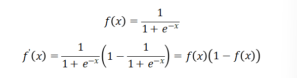
1.1 Sigmoid函数

PyTorch中已经实现了神经网络中可能用到的各种激活函数，我们在代码中只要直接调用即可。

表示二分类概率

import torch
import matplotlib.pyplot as pltx = torch.linspace(-10, 10, 1000, requires_grad=True)
fig, ax = plt.subplots(1, 2)
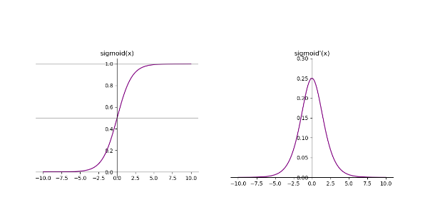
fig.set_size_inches(12, 4)ax[0].plot(x.data, torch.sigmoid(x).data, "purple")
ax[0].set_title("sigmoid(x)")
ax[0].spines["top"].set_visible(False)#上边界不可见
ax[0].spines["right"].set_visible(False)
ax[0].spines["left"].set_position("zero")#左边界放在0的位置
ax[0].spines["bottom"].set_position("zero")
ax[0].axhline(0.5, color="gray", alpha=0.7, linewidth=1)#画横线
ax[0].axhline(1, color="gray", alpha=0.7, linewidth=1)torch.sigmoid(x).sum().backward() # 反向传播计算梯度
ax[1].plot(x.data, x.grad, "purple")
ax[1].set_title("sigmoid'(x)")
ax[1].spines["top"].set_visible(False)
ax[1].spines["right"].set_visible(False)
ax[1].spines["left"].set_position("zero")
ax[1].spines["bottom"].set_position("zero")
ax[1].set_ylim(0, 0.3)plt.show()

1.2 Tanh函数

import torch
import matplotlib.pyplot as pltx = torch.linspace(-5, 5, 1000, requires_grad=True)
fig, ax = plt.subplots(1, 2)
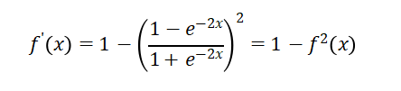
fig.set_size_inches(12, 4)ax[0].plot(x.data, torch.tanh(x).data, "purple")
ax[0].set_title("tanh(x)")
ax[0].spines["top"].set_visible(False)
ax[0].spines["right"].set_visible(False)
ax[0].spines["left"].set_position("zero")
ax[0].spines["bottom"].set_position("zero")
ax[0].axhline(-1, color="gray", alpha=0.7, linewidth=1)
ax[0].axhline(1, color="gray", alpha=0.7, linewidth=1)torch.tanh(x).sum().backward() # 反向传播计算梯度
ax[1].plot(x.data, x.grad, "purple")
ax[1].set_title("tanh'(x)")
ax[1].spines["top"].set_visible(False)
ax[1].spines["right"].set_visible(False)
ax[1].spines["left"].set_position("zero")
ax[1].spines["bottom"].set_position("zero")plt.show()

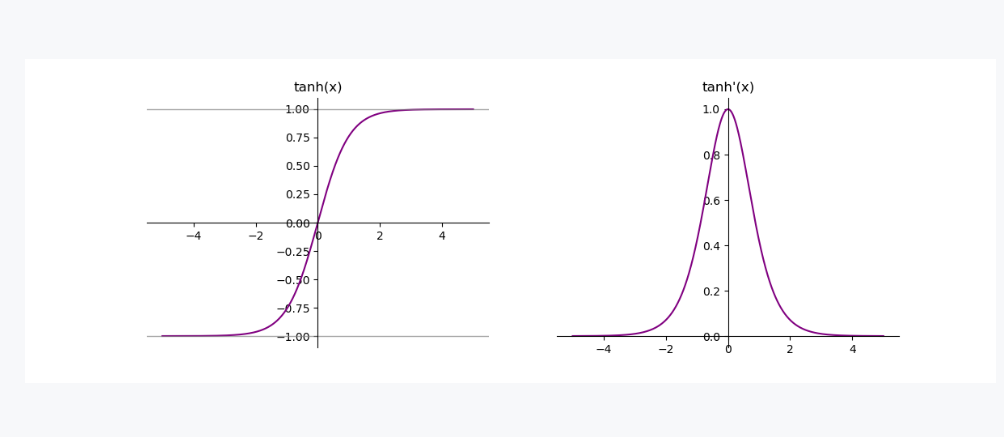
这两个函数在反向传播的时候，都容易出现梯度消失的情况，都是用于二分类

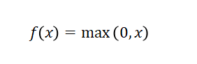
1.3 ReLU函数

import torch
import matplotlib.pyplot as pltx = torch.linspace(-5, 5, 1000, requires_grad=True)
fig, ax = plt.subplots(1, 2)
fig.set_size_inches(12, 4)ax[0].plot(x.data, torch.relu(x).data, "purple")
ax[0].set_title("relu(x)")
ax[0].spines["top"].set_visible(False)
ax[0].spines["right"].set_visible(False)
ax[0].spines["left"].set_position("zero")
ax[0].spines["bottom"].set_position("zero")torch.relu(x).sum().backward()  # 反向传播计算梯度
ax[1].plot(x.data, x.grad, "purple")
ax[1].set_title("relu'(x)")
ax[1].spines["top"].set_visible(False)
ax[1].spines["right"].set_visible(False)
ax[1].spines["left"].set_position("zero")
ax[1].spines["bottom"].set_position("zero")plt.show()

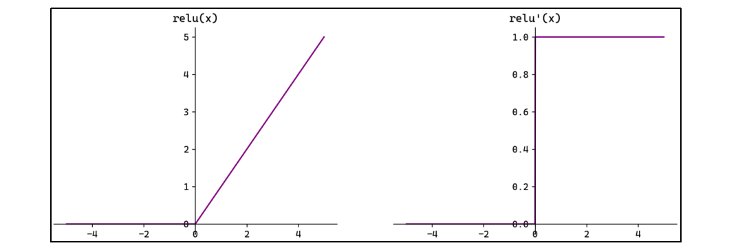
这个是用于回归问题，转换出来不变

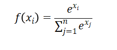
1.4 Softmax函数

这个是用于多分类

x = torch.randn(3,5)
print(x)

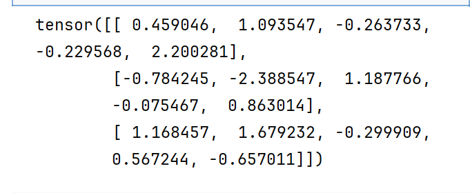
y = torch.softmax(x,dim=1)
print(y)

大的数概率就比较大了

2. 参数初始化和正则化

2.1 全连接层（nn.Linear）–线性层

在神经网络中，参数主要位于全连接层（仿射层Affine）中。
PyTorch提供了torch.nn模块，专门用于神经网络的构建和训练。其中全连接层被实现为Linear类，内部有两个属性：权重 weight和偏置bias；这就是神经网络的主要参数。

权重 weight和偏置bias–》要初始化好，不然一开始就训练不好

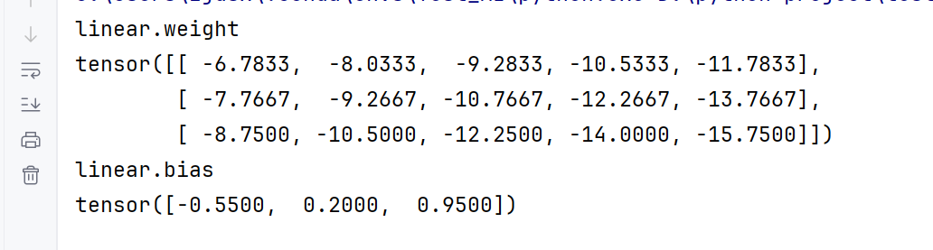
import torch.nn as nnlinear = nn.Linear(5, 2)

上面代码定义了一个有5个输入神经元、2个输出神经元的全连接层。

2.2 常数初始化

所有权重参数初始化为一个常数。

#定义一个全连接层
linear = nn.Linear(5,2)

#常数初始化
nn.init.zeros_(linear.weight)
print(linear.weight)

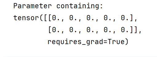
默认打开了requires_grad=True

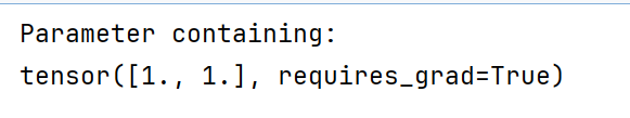
nn.init.ones_(linear.bias)
print(linear.bias)

nn.init.constant_(linear.weight,10)
print(linear.weight)

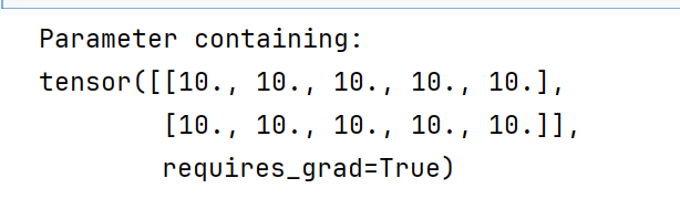
发现变成2*5了

默认转置了，因为反向传播和前向传播的时候就要转置，所以就先转置了

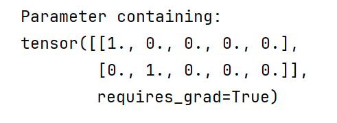
2.3 秩初始化

nn.init.eye_(linear.weight)

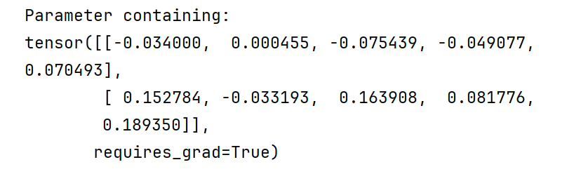
2.4 正态分布初始化

nn.init.normal_(linear.weight,mean=0,std=0.1)

2.5 均匀分布初始化

nn.init.uniform_(linear.weight,a=-1,b=1)

2.6 Xavier初始化（Glorot初始化）

Xavier初始化根据输入和输出的神经元数量调整权重的初始范围，确保每一层的输出方差与输入方差相近。适用于Sigmoid和Tanh等激活函数，能有效缓解梯度消失或爆炸问题。

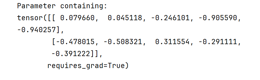
nn.init.xavier_normal_(linear.weight)
nn.init.xavier_uniform_(linear.weight)

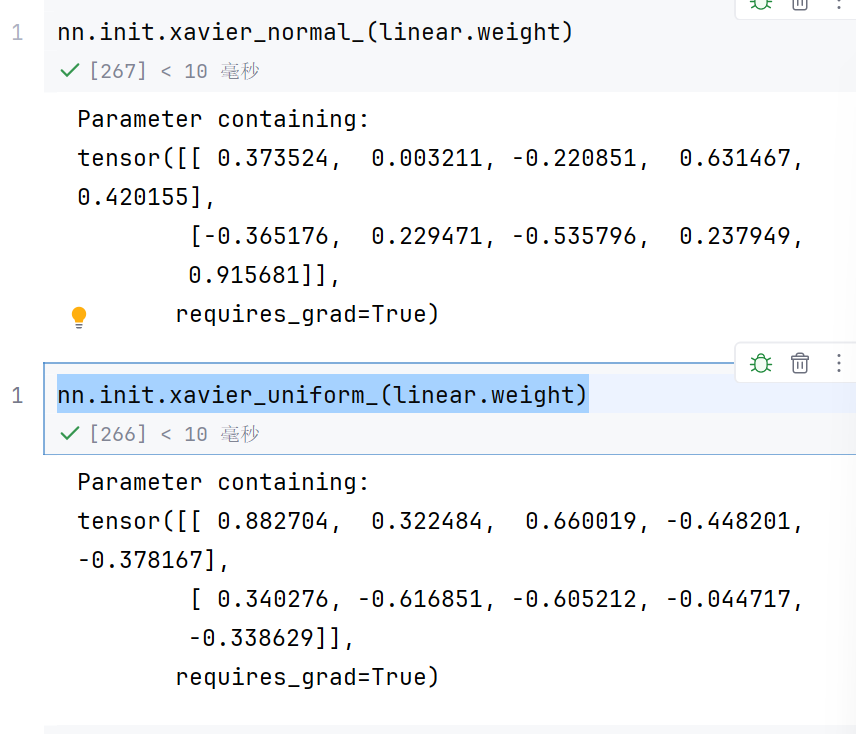
这个用于sigmoid，Ranh

2.7 He初始化（Kaiming初始化）

用于ReLU

He初始化根据输入的神经元数量调整权重的初始范围。主要适用于ReLU及其变体（如Leaky ReLU）激活函数。

nn.init.kaiming_normal_(linear.weight)
nn.init.kaiming_uniform_(linear.weight)

2.8 Dropout随机失活

Dropout（随机失活，暂退法）是一种在学习的过程中随机关闭神经元的方法。
可以通过torch.nn.Dropout§来使用Dropout，并通过参数p来设置失活概率。

x = torch.randint(1,10,(10,))

#定义一个Dropout层
dropout = nn.Dropout(p=0.5)
y = dropout(x)

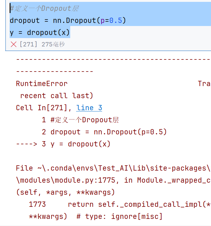
这里报错的原因主要是因为类型不匹配，要用float类型

x = torch.randint(1,10,(10,),dtype=torch.float32)

#定义一个Dropout层
dropout = nn.Dropout(p=0.5)
y = dropout(x)
print(x)
print(y)

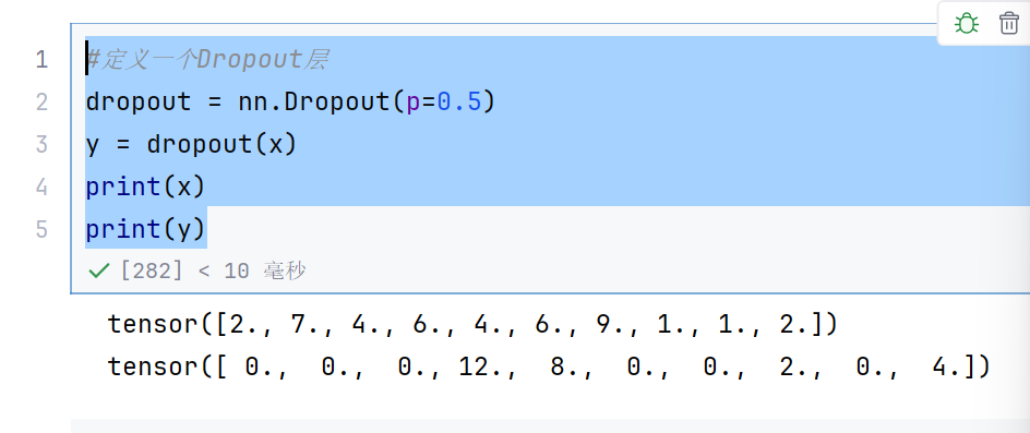
0表示关闭的神经元，没有关闭的神经元就放大为原来的两倍

3. 搭建神经网络

3.1 自定义模型

在神经网络框架中，由多个层组成的组件称之为 模块（Module）。
在PyTorch中模型就是一个Module，各网络层、模块也是Module。Module是所有神经网络的基类。
在定义一个Module时，我们需要继承torch.nn.Module并主要实现两个方法：
__init__：定义网络各层的结构，并初始化参数。
forward：根据输入进行前向传播，并返回输出。计算其输出关于输入的梯度，可通过其反向传播函数进行访问（通常自动发生）。forward方法是每次调用的具体实现。
接下来使用PyTorch实现下图的神经网络：

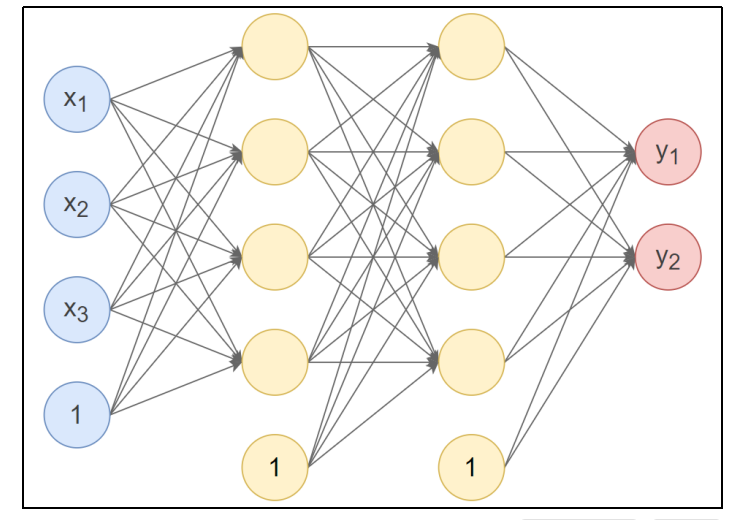
反向传播不需要定义，因为前向弄好了，反向就自动OK了

第1个隐藏层：使用Xavier正态分布初始化权重，激活函数使用Tanh。
第2个隐藏层：使用He正态分布初始化权重，激活函数使用ReLU。
输出层：按默认方式初始化，激活函数使用Softmax。

import torch
import torch.nn as nn#自定义神经网络类class Model(nn.Module):#初始化def __init__(self):super().__init__()#定义三个线性层self.linear1 = nn.Linear(3,4)# 线性层w和b的参数初始化nn.init.xavier_normal_(self.linear1.weight)self.linear2 = nn.Linear(4, 4)nn.init.kaiming_normal_(self.linear2.weight)self.out = nn.Linear(4, 2)# 前向传播def forward(self, x):x = self.linear1(x)x = torch.tanh(x)x = self.linear2(x)x = torch.relu(x)x = self.out(x)x = torch.softmax(x,dim=1)return x#测试，定义数据
model = Model()
x = torch.randn(10,3)
output = model(x)
print("神经网络输出",output)

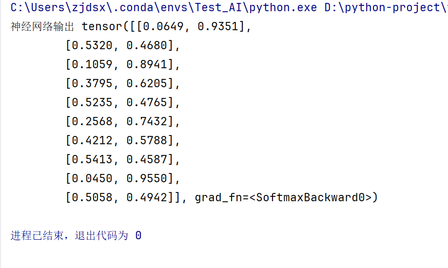
输入103，输出102，表示每个特征的概率
这个神经并没有训练模型的

3.2 查看模型参数

print(model.linear1.weight)
print(model.linear1.bias)
print(model.linear2.weight)
print(model.linear2.bias)
print(model.out.weight)
print(model.out.bias)

但是这样比较麻烦

for param in model.parameters():print(param)

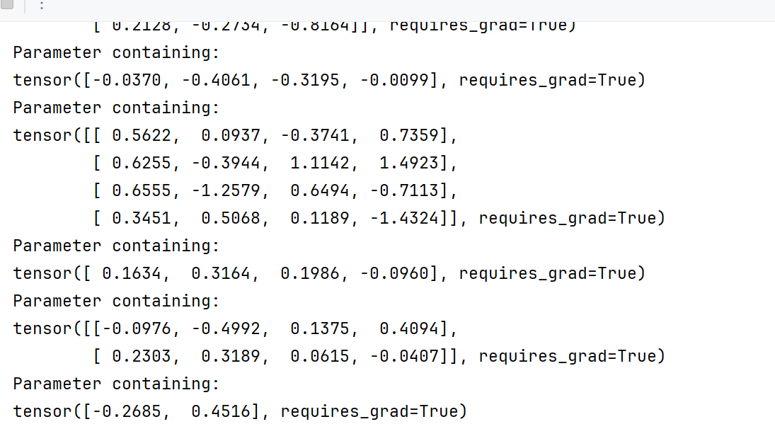
但是还是不知道哪个层是哪个的

for param in model.named_parameters():print(param)

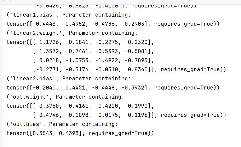
这样就知道谁是谁了

print(model.state_dict())

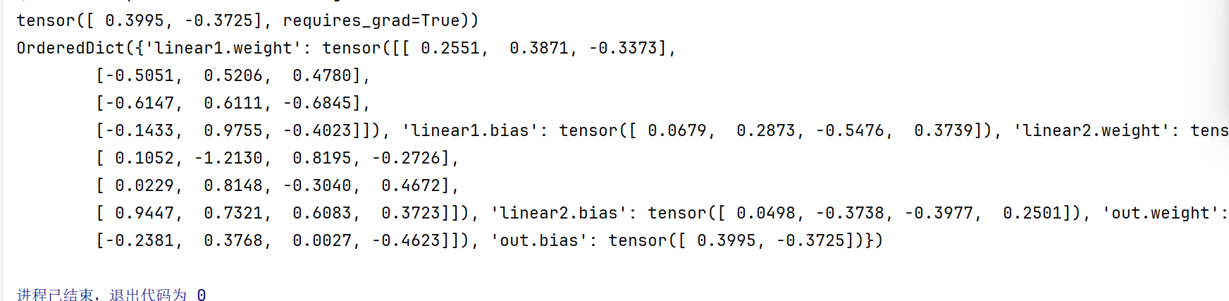
这个就是把模型参数用一个字典的形式存储，更加方便了

3.3 查看模型结构和参数数量

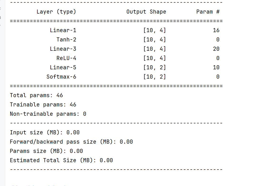
可使用torchsummary.summary来查看模型结构与参数数量。需要先安装torchsummary库：pip install torchsummary。

from torchsummary import summary
# input_size表示输入神经元个数为3---》特征个数
#batch_size表示个数，有多少个东西
# device表示使用cpu运行
summary(model,input_size=(3,),batch_size=10,device='cpu')

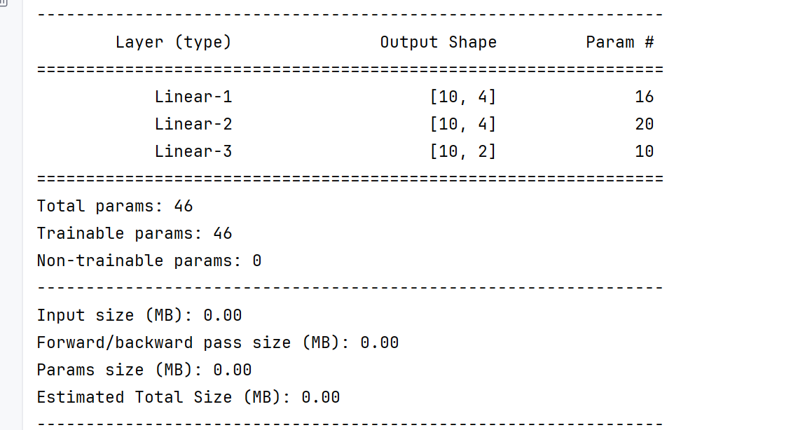
Param #表示每一层的参数个数
比如第一层
w为3*4
b为4
所以就是16个

1B就是10亿个参数
deepseek有671B个参数，满血版

3.4 device设置

cpu计算能力比gpu强
但是gpu对并行运算有架构优化

gpu=1000个小学生
cpu=1个博士生

同时去算10000道十以内数学题—》小学生胜利

gpu做简单任务—》快
cpu做复杂任务

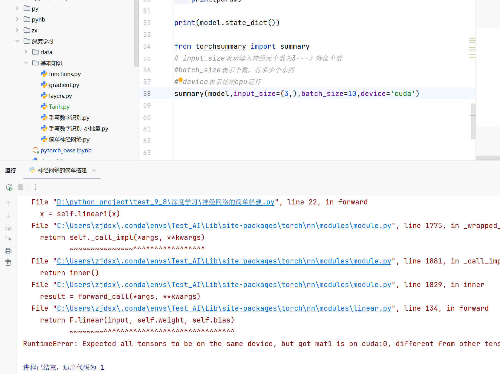
但是直接改为cuda，就报错了
因为前面的张量是在cpu上运行的

现在又在显卡上，gpu上运行—》不行

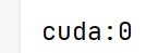
input = torch.randn(1,5,device='cuda')
print(input.device)

input = torch.randn(1,5,device='cuda').to(device='cpu')
print(input.device)

发现设备还可以转换的

import torch
import torch.nn as nn#自定义神经网络类class Model(nn.Module):#初始化def __init__(self):super().__init__()#定义三个线性层self.linear1 = nn.Linear(3,4,device='cuda')# 线性层w和b的参数初始化nn.init.xavier_normal_(self.linear1.weight)self.linear2 = nn.Linear(4, 4,device='cuda')nn.init.kaiming_normal_(self.linear2.weight)self.out = nn.Linear(4, 2,device='cuda')# 前向传播def forward(self, x):x = self.linear1(x)x = torch.tanh(x)x = self.linear2(x)x = torch.relu(x)x = self.out(x)x = torch.softmax(x,dim=1)return x#测试，定义数据
model = Model()
x = torch.randn(10,3,device='cuda')
output = model(x)
print("神经网络输出",output)print(model.linear1.weight)
print(model.linear1.bias)
print(model.linear2.weight)
print(model.linear2.bias)
print(model.out.weight)
print(model.out.bias)for param in model.parameters():print(param)for param in model.named_parameters():print(param)print(model.state_dict())from torchsummary import summary
# input_size表示输入神经元个数为3---》特征个数
#batch_size表示个数，有多少个东西
# device表示使用cpu运行
summary(model,input_size=(3,),batch_size=10,device='cuda')

这样给每一个类都弄上device就没有问题了—》张量和线性层
—》张量麻烦，因为有很多层

class Model(nn.Module):#初始化def __init__(self,device='cpu'):super().__init__()#定义三个线性层self.linear1 = nn.Linear(3,4,device=device)# 线性层w和b的参数初始化nn.init.xavier_normal_(self.linear1.weight)self.linear2 = nn.Linear(4, 4,device=device)nn.init.kaiming_normal_(self.linear2.weight)self.out = nn.Linear(4, 2,device=device)

#测试，定义数据
model = Model(device='cuda')

可以在构造函数那里指定device

#自定义神经网络类class Model(nn.Module):#初始化def __init__(self,device='cpu'):super().__init__()#定义三个线性层self.linear1 = nn.Linear(3,4,device=device)# 线性层w和b的参数初始化nn.init.xavier_normal_(self.linear1.weight)self.linear2 = nn.Linear(4, 4,device=device)nn.init.kaiming_normal_(self.linear2.weight)self.out = nn.Linear(4, 2,device=device)# 前向传播def forward(self, x):x = self.linear1(x)x = torch.tanh(x)x = self.linear2(x)x = torch.relu(x)x = self.out(x)x = torch.softmax(x,dim=1)return x#统一定义全景变量device
device = 'cuda' if torch.cuda.is_available() else 'cpu'#测试，定义数据
model = Model(device=device)
x = torch.randn(10,3,device=device)
output = model(x)
print("神经网络输出",output)print(model.linear1.weight)
print(model.linear1.bias)
print(model.linear2.weight)
print(model.linear2.bias)
print(model.out.weight)
print(model.out.bias)for param in model.parameters():print(param)for param in model.named_parameters():print(param)print(model.state_dict())from torchsummary import summary
# input_size表示输入神经元个数为3---》特征个数
#batch_size表示个数，有多少个东西
# device表示使用cpu运行
summary(model,input_size=(3,),batch_size=10,device=device)

这样也是一样的，给一个全局变量

3.5 使用Sequential构建模型

可以通过torch.nn.Sequential来构建模型，将各层按顺序传入。

import torch
import torch.nn as nn
from torchsummary  import summary#定义数据
x = torch.randn(10,3)
#构建模型
model = nn.Sequential(nn.Linear(3,4),nn.Tanh(),nn.Linear(4,4),nn.ReLU(),nn.Linear(4,2),nn.Softmax(dim=1),
)
#定义一个参数初始化函数
def init_params(layer):if isinstance(layer, nn.Linear):nn.init.xavier_uniform_(layer.weight)nn.init.constant_(layer.bias,0.1)#参数初始化
model.apply(init_params)#前向传播
output = model(x)
print(output)
summary(model,input_size=(3,),batch_size=10,device='cpu')

这样就把激活层都当做线性层了–》也可以

4. 损失函数

4.1 二分类任务损失函数

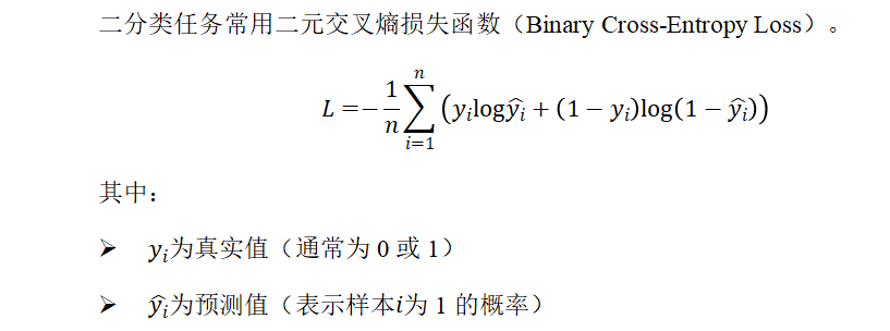
1）二分类任务损失函数
在PyTorch中可使用torch.nn.BCELoss实现：

#%%
#输入数据
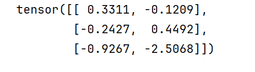
input = torch.randn(3,2)
print(input)

#目标值
target = torch.tensor([[0,1],[1,0],[0,1]],dtype=torch.float)

因为后面会进行运算，所以要用浮点数

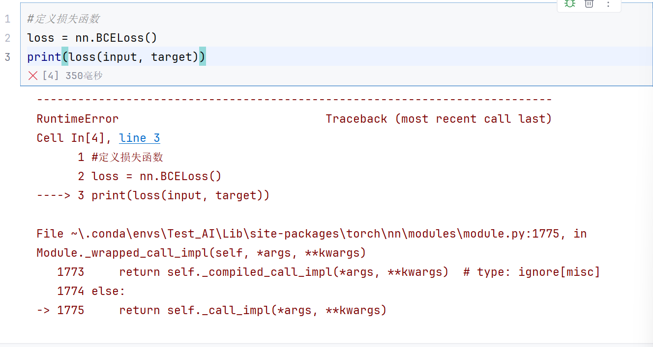
这样肯定是不行的，因为input不是预测1的概率值

#输入数据
input = torch.randn(3,2)
print(input)
pred = torch.sigmoid(input)
print(pred)

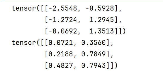
因为sigmoid生成的就是0~1，所以可以用它来生成预测值

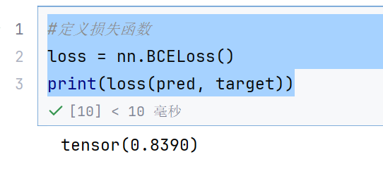
#定义损失函数
loss = nn.BCELoss()
print(loss(pred, target))

4.2 多分类任务损失函数

2）多分类任务损失函数

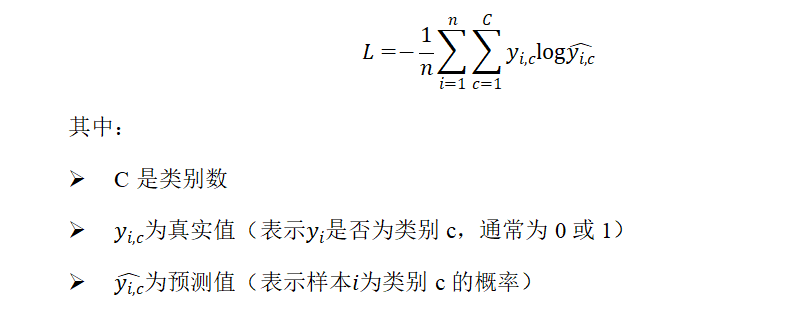
多分类任务常用多类交叉熵损失函数（Categorical Cross-Entropy Loss）。它是对每个类别的预测概率与真实标签之间差异的加权平均。

在PyTorch中可使用torch.nn.CrossEntropyLoss 实现：

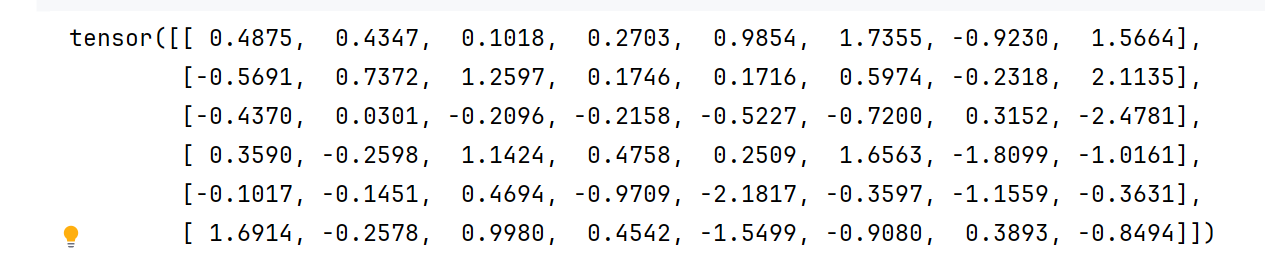
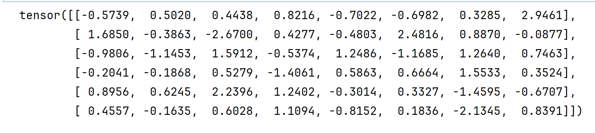
input = torch.randn(6,8)
print(input)

#目标值，6个数据的类别标签
target = torch.tensor([1,0,3,7,5,2])

pred = torch.softmax(input,dim=1)
print(pred)

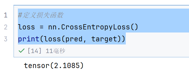
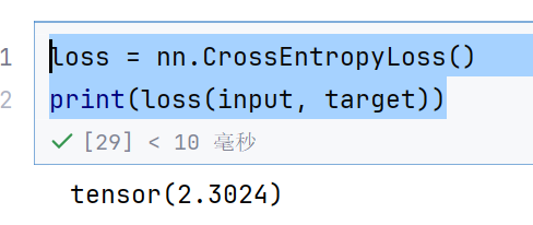
#定义损失函数
loss = nn.CrossEntropyLoss()
print(loss(pred, target))

#定义损失函数
loss = nn.CrossEntropyLoss()
print(loss(input, target))

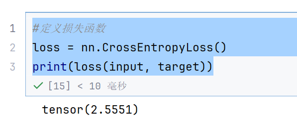
我们还可以直接传入input—》因为这个函数进行处理的了
注意：调用torch.nn.CrossEntropyLoss相当于调用了torch.nn.LogSoftmax之后再调用torch.nn.NLLLoss。即使用CrossEntropyLoss时上一层的输出不需要Softmax激活函数，因为该损失函数内会自动处理。
8指的是8个类别
pred是预测的每个类别的概率

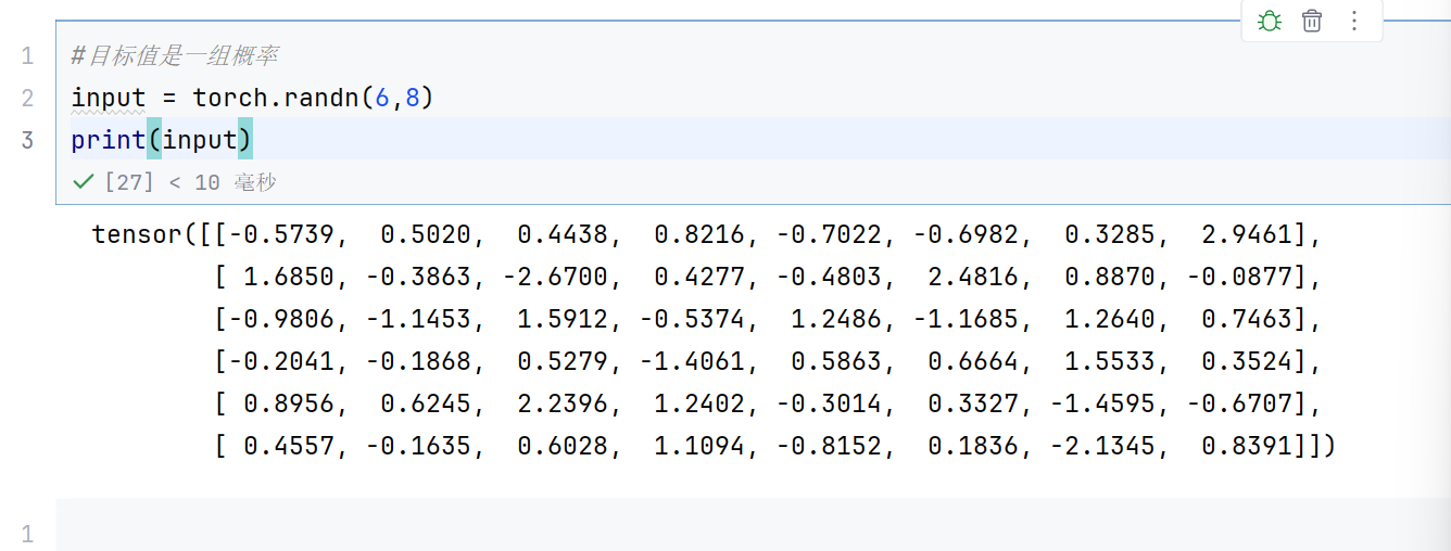
目标值是一组概率

target = torch.randn(6,8).softmax(dim=1)
print(input)

loss = nn.CrossEntropyLoss()
print(loss(input, target))

所以目标值是概率值还是类别标签都是可以计算的

4.3 回归任务损失函数

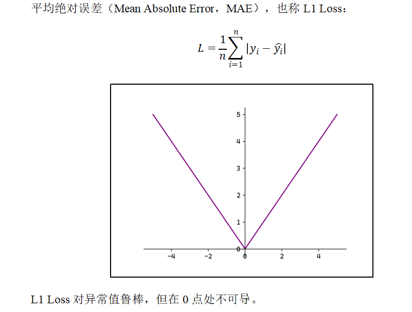
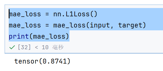
1）MAE

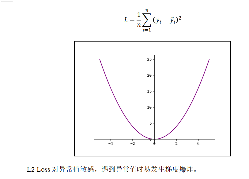
2）MSE

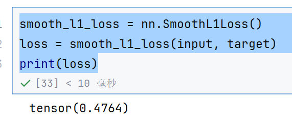
3）Smooth L1

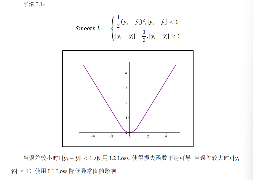
#回归
input = torch.randn(3,5)
target = torch.randn(3,5)

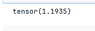
mse_loss = nn.MSELoss()
mse_loss = mse_loss(input, target)
print(mse_loss)

mae_loss = nn.L1Loss()
mae_loss = mae_loss(input, target)
print(mae_loss)

smooth_l1_loss = nn.SmoothL1Loss()
loss = smooth_l1_loss(input, target)
print(loss)

4.4 损失函数综合测试

import torch
from torch import nn,optim#定义模型
class Model(nn.Module):def __init__(self):super().__init__()#只定义一个全连接层---》线性层self.linear = nn.Linear(5,3)#权值初始化self.linear.weight.data = torch.tensor([[0.1,0.2,0.3],[0.4,0.5,0.6],[0.7,0.8,0.9],[1.0,1.1,1.2],[1.3,1.4,1.5],]).Tself.linear.bias.data = torch.tensor([1.0,2.0,3.0])def forward(self, x):return self.linear(x)return x#输入数据2*5
X = torch.tensor([[1,2,3,4,5],[6,7,8,9,10]],dtype=torch.float32)
#目标值2*3
target = torch.tensor([[0,0,0],[0,0,0]],dtype=torch.float32)
#创建模型
model = Model()
#前向传播
output = model(X)
#定义损失函数
loss =  nn.MSELoss()
loss_value = loss(output, target)#反向传播计算梯度
loss_value.backward()# 定义优化器
optimizer = optim.SGD(model.parameters(), lr=0.1)
#更新参数w和b
optimizer.step()
# 清除梯度，再次迭代
optimizer.zero_grad()#打印模型参数
for param in model.state_dict():print(param)print(model.state_dict()[param])

总结