基于frenet坐标系的规划与避障
目录
- 1. 概述
- 1.1 什么是Frenet坐标系
- 1.2 Frenet坐标系的优势
- 步骤
- 步骤1:坐标转换
- 笛卡尔与Frenet坐标转换
- 步骤2:采样目标生成
- 横向目标采样
- 速度采样
- 时间采样
- 步骤3计算多项式参数
- 步骤4 采样得到最终轨迹
基于frenet坐标系的规划,如果不加入感知信息,那么采样的轨迹就像是这样的:
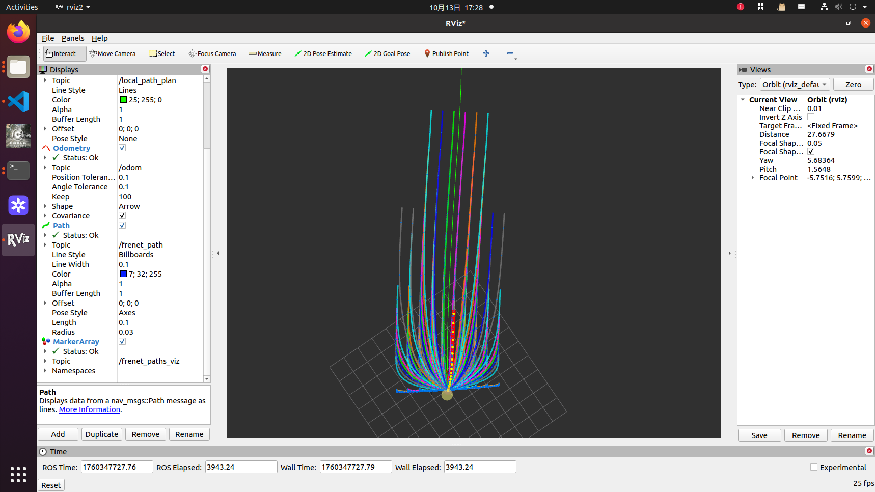
以上内容后续再整理出来,我们今天主要从数学原理上理解这整个过程。
1. 概述
1.1 什么是Frenet坐标系
Frenet坐标系是一种沿着参考路径的自然坐标系,由法国数学家Jean Frédéric Frenet提出。在自动驾驶路径规划中,Frenet坐标系将复杂的二维路径规划问题分解为两个相对独立的一维问题:
-
纵向规划(s方向):沿着参考路径的运动规划
-
横向规划(d方向):垂直于参考路径的偏移规划
1.2 Frenet坐标系的优势
- 问题解耦:将2D路径规划分解为两个1D问题
- 直观性强:更符合驾驶员的思维模式
- 约束简化:道路边界、车道线等约束在Frenet坐标系中更容易表达
- 计算效率:降低了计算复杂度
s: 沿参考路径的累积弧长(纵向位置)
d: 垂直于参考路径的横向偏移(正值表示左侧,负值表示右侧)
步骤
输入包括两个方面,一个是车辆当前的定位,一个是参考路径。
接下来我们是需要对完整的过程进行分析的
步骤1:坐标转换
将车辆当前状态从笛卡尔坐标系转换到Frenet坐标系:
-
输入:
(x, y, θ, v) -
输出:
(s, d, s_dot, d_dot, s_ddot, d_ddot)
笛卡尔与Frenet坐标转换
参考线首先需要进行处理
关键计算步骤:
- 切线向量计算:使用差分方法计算路径切线方向
- 法向量计算:将切线向量逆时针旋转90度得到法向量
- 向量归一化:确保向量长度为1,便于后续计算
def _precompute_path_properties(self):"""预计算参考路径属性"""self.tangent_vectors = []self.normal_vectors = []for i in range(len(self.reference_path)):if i == 0:# 第一个点:使用向前差分dx = self.reference_path[i+1].x - self.reference_path[i].xdy = self.reference_path[i+1].y - self.reference_path[i].yelif i == len(self.reference_path) - 1:# 最后一个点:使用向后差分dx = self.reference_path[i].x - self.reference_path[i-1].xdy = self.reference_path[i].y - self.reference_path[i-1].yelse:# 中间点:使用中心差分dx = self.reference_path[i+1].x - self.reference_path[i-1].xdy = self.reference_path[i+1].y - self.reference_path[i-1].y# 归一化切线向量length = math.sqrt(dx**2 + dy**2)if length > 1e-6:tangent = (dx/length, dy/length)normal = (-dy/length, dx/length) # 逆时针旋转90度else:tangent = (1.0, 0.0)normal = (0.0, 1.0)self.tangent_vectors.append(tangent)self.normal_vectors.append(normal)
然后是笛卡尔坐标系转到frenet坐标系
def cartesian_to_frenet(self, x: float, y: float) -> Tuple[float, float]:"""笛卡尔坐标转Frenet坐标"""if not self.reference_path:return 0.0, 0.0# 1. 寻找最近参考点min_distance = float('inf')closest_index = 0for i, ref_point in enumerate(self.reference_path):distance = math.sqrt((x - ref_point.x)**2 + (y - ref_point.y)**2)if distance < min_distance:min_distance = distanceclosest_index = i# 2. 计算投影ref_point = self.reference_path[closest_index]# 从参考点到目标点的向量dx = x - ref_point.xdy = y - ref_point.y# 投影到切线方向(s方向)tangent = self.tangent_vectors[closest_index]s_projection = dx * tangent[0] + dy * tangent[1]# 投影到法线方向(d方向)normal = self.normal_vectors[closest_index]d = dx * normal[0] + dy * normal[1]# 3. 计算最终的s坐标s = ref_point.s + s_projectionreturn s, d
向量PR = (x-x_r, y-y_r)
切线向量T = (t_x, t_y)
法向量N = (n_x, n_y)s_offset = PR · T = (x-x_r)*t_x + (y-y_r)*t_y
d = PR · N = (x-x_r)*n_x + (y-y_r)*n_y
s = s_r + s_offset
d = d (横向偏移)
def frenet_to_cartesian(self, s: float, d: float) -> Tuple[float, float]:"""Frenet坐标转笛卡尔坐标"""# 确保s在有效范围内s = max(0.0, min(s, self.path_length))# 通过插值找到s对应的参考点ref_point, ref_index = self._interpolate_reference_point(s)# 计算笛卡尔坐标normal_vec = self.normal_vectors[ref_index]x = ref_point.x + d * normal_vec[0]y = ref_point.y + d * normal_vec[1]return x, y
P(x,y) = R(x_r,y_r) + d * N(n_x,n_y)
x = x_r + d * n_x
y = y_r + d * n_y
很多人可能理解不了参考线上的匹配点为什么不能直接使用,因为对于最小距离来说,并不一定是垂直关系:

很明显,我们真正要求的s还有一段,所以s = s_r + s_offset
步骤2:采样目标生成
基于path_sampler.py,系统采用三维采样策略:
- 横向采样:在参考线两侧生成不同的横向偏移目标
- 速度采样:生成不同的目标速度
- 时间采样:生成不同的规划时间长度
横向目标采样
def _generate_lateral_targets(self, current_d: float) -> List[float]:"""生成横向采样目标"""targets = []if self.config.weights.lateral_sample_num <= 1:targets.append(0.0) # 只采样参考线else:# 在[-lateral_sample_range, +lateral_sample_range]范围内均匀采样range_val = self.config.weights.lateral_sample_rangenum_samples = self.config.weights.lateral_sample_numfor i in range(num_samples):if num_samples == 1:lateral_offset = 0.0else:# 均匀分布采样ratio = i / (num_samples - 1)lateral_offset = -range_val + 2 * range_val * ratiotargets.append(lateral_offset)return targets
-
配置参数:
lateral_sample_range = 3.0m,lateral_sample_num = 5 -
生成目标:
[-3.0, -1.5, 0.0, 1.5, 3.0]
2.3 速度和时间采样
def _generate_longitudinal_targets(self) -> List[Tuple[float, float]]:"""生成纵向采样目标(速度, 时间)"""targets = []# 速度采样speed_targets = []if self.config.weights.speed_sample_num <= 1:speed_targets.append(self.reference_speed)else:base_speed = self.reference_speedspeed_range = self.config.weights.speed_sample_rangefor i in range(self.config.weights.speed_sample_num):ratio = i / (self.config.weights.speed_sample_num - 1)speed = base_speed - speed_range/2 + speed_range * ratiospeed = max(0.1, speed) # 确保速度为正speed_targets.append(speed)# 时间采样time_targets = []if self.config.weights.time_sample_num <= 1:time_targets.append(self.config.planning_horizon)else:base_time = self.config.planning_horizontime_range = self.config.weights.time_sample_rangefor i in range(self.config.weights.time_sample_num):ratio = i / (self.config.weights.time_sample_num - 1)time = base_time - time_range/2 + time_range * ratiotime = max(0.5, time) # 确保时间为正time_targets.append(time)# 组合所有目标for speed in speed_targets:for time in time_targets:targets.append((speed, time))return targets
速度采样
配置参数:
- speed_sample_range = 5.0 m/s
- speed_sample_num = 5
- target_speed = 2.0 m/s (基准速度)
base_speed = 2.0 # 基准速度
speed_range = 5.0 # 采样范围
speed_num = 5 # 采样数量
# 生成速度目标:从(2.0-5.0)到(2.0+5.0),即-3.0到7.0
# 但要确保速度为正,所以最小值是0.1
速度目标 = [0.1, 1.5, 2.0, 4.5, 7.0]  # (经过正值限制)
时间采样
配置参数:
- time_sample_range = 2.0s
- time_sample_num = 5
- planning_horizon = 5.0s (基准时间)
base_time = 5.0 # 基准规划时间
time_range = 2.0 # 采样范围
time_num = 5 # 采样数量
# 生成时间目标:从(5.0-2.0)到(5.0+2.0),即3.0到7.0
时间目标 = [3.0, 4.0, 5.0, 6.0, 7.0]
步骤3计算多项式参数
最终的采样目标是125条组合,这些组合可以构成多项式的目标状态。
- 横向目标 : 5个 [-2.5, -1.25, 0.0, 1.25, 2.5]
- 速度目标 : 5个 [0.1, 1.5, 2.0, 4.5, 7.0]
- 时间目标 : 5个 [3.0, 4.0, 5.0, 6.0, 7.0]
总候选轨迹数 : 5 × 5 × 5 = 125条候选轨迹
由以上的采样组合就可以计算出一系列的终态目标了。
例如
# 采样目标
lateral_target = 1.25  # 横向采样目标位置# 当前车辆状态
start_state = VehicleState(s=0.0,      # 当前纵向位置d=0.0,      # 当前横向位置  s_dot=2.0,  # 当前纵向速度d_dot=0.0,  # 当前横向速度s_ddot=0.0, # 当前纵向加速度d_ddot=0.0  # 当前横向加速度
)# 规划参数
planning_time = 5.0  # 规划时间
planning_distance = start_state.s_dot * planning_time  # 规划距离 = 2.0 * 5.0 = 10.0米# 横向多项式的目标状态
横向目标状态 = {'s0': start_state.s,           # 起始纵向位置 = 0.0's1': start_state.s + planning_distance,  # 终止纵向位置 = 0.0 + 10.0 = 10.0'd0': start_state.d,           # 起始横向位置 = 0.0'd1': lateral_target,          # 终止横向位置 = 1.25 (采样目标)'dd0': start_state.d_dot,      # 起始横向速度 = 0.0'dd1': 0.0,                    # 终止横向速度 = 0.0 (设定为0,表示平稳到达)'ddd0': start_state.d_ddot,    # 起始横向加速度 = 0.0'ddd1': 0.0                    # 终止横向加速度 = 0.0 (设定为0,表示平稳到达)
}
对于纵向目标状态
# 采样目标
target_speed = 4.5   # 目标速度采样值
planning_time = 5.0  # 规划时间采样值# 纵向多项式的目标状态
纵向目标状态 = {'s0': start_state.s,           # 起始纵向位置 = 0.0'v0': start_state.s_dot,       # 起始速度 = 2.0'a0': start_state.s_ddot,      # 起始加速度 = 0.0'target_speed': target_speed,   # 终止速度 = 4.5 (采样目标)'T': planning_time             # 规划时间 = 5.0 (采样目标)
}
然后是根据这些终态信息和初始信息来计算所有的多项式的参数
对于方程组来说,列出:
# 五次多项式:d(t) = a0 + a1*t + a2*t² + a3*t³ + a4*t⁴ + a5*t⁵
# 其中 t 是归一化参数 [0,1]# 6个约束条件:
# d(0) = a0 = 0                           → a0 = 0
# d(1) = a0 + a1 + a2 + a3 + a4 + a5 = 1.25
# d'(0) = a1 = 0                          → a1 = 0
# d'(1) = a1 + 2a2 + 3a3 + 4a4 + 5a5 = 0
# d''(0) = 2a2 = 0                        → a2 = 0
# d''(1) = 2a2 + 6a3 + 12a4 + 20a5 = 0
对应求解时,我们通过矩阵实现
import numpy as npA = np.array([[1, 0, 0, 0, 0, 0],      # d(0) = 0[1, 1, 1, 1, 1, 1],      # d(1) = 1.25[0, 1, 0, 0, 0, 0],      # d'(0) = 0[0, 1, 2, 3, 4, 5],      # d'(1) = 0[0, 0, 2, 0, 0, 0],      # d''(0) = 0[0, 0, 2, 6, 12, 20]     # d''(1) = 0
])b = np.array([0, 1.25, 0, 0, 0, 0])
coeffs = np.linalg.solve(A, b)
# 结果: [0, 0, 0, 10, -15, 6]
得到
d(t) = 0 + 0*t + 0*t² + 10*t³ - 15*t⁴ + 6*t⁵= 10t³ - 15t⁴ + 6t⁵
同样的,三次多项式的约束条件列出来
带入已知来求解即可
s(t) = 0 + 2.0*t + 0*t² + 0.0333*t³= 2.0*t + 0.0333*t³``````python
# 三次多项式:s(t) = a0 + a1*t + a2*t² + a3*t³
# 4个约束条件:
# s(0) = a0 = 0                    → a0 = 0
# s'(0) = a1 = 2.0                 → a1 = 2.0
# s''(0) = 2a2 = 0                 → a2 = 0
# s'(T) = a1 + 2a2*T + 3a3*T² = 4.5
步骤4 采样得到最终轨迹
最后的步骤,需要对求出的多项式进行最终采样,得到轨迹和速度信息
# 假设规划时间T=5.0秒,时间步长dt=0.1秒
for t in [0, 0.1, 0.2, ..., 5.0]:# 1. 从纵向多项式获得位置和速度s = 2.0*t + 0.0333*t³s_dot = 2.0 + 3*0.0333*t²  # 对时间求导s_ddot = 6*0.0333*t        # 对时间二阶求导# 2. 从横向多项式获得横向位置(需要归一化时间)t_norm = t / 5.0  # 归一化到[0,1]d = 10*t_norm³ - 15*t_norm⁴ + 6*t_norm⁵d_dot = (30*t_norm² - 60*t_norm³ + 30*t_norm⁴) / 5.0  # 对s求导再除以ds/dt# 3. 转换为笛卡尔坐标x, y = frenet_to_cartesian(s, d)# 4. 生成轨迹点trajectory_point = FrenetPoint(s, d, s_dot, d_dot, s_ddot, d_ddot, x, y, ...)
【一些不重要的实车开发过程记录】
原仿真是在ros1 noetic下进行的
[INFO] [1757827166.480113, 740.760000]: delta : -3.997965
STOP
STOP
STOP
STOP
STOP
[INFO] [1757827166.493232, 740.769000]: kp is : 7026.709727
[ERROR] [1757827166.493309, 740.769000]: bad callback: <function callback_feedback at 0x7f0ea6a17550>
Traceback (most recent call last):File "/opt/ros/noetic/lib/python3/dist-packages/rospy/topics.py", line 750, in _invoke_callbackcb(msg)File "/home/cyun/9.13/sim/src/Frenet_Planner_Simulation/tracking_control/src/scripts/tracking_Methods/pure_pursuit.py", line 89, in callback_feedbackep = min(distances)
ValueError: min() arg is an empty sequenceSTOP
[INFO] [1757827166.494130, 740.769000]: ki is : 5401.404924
[INFO] [1757827166.494902, 740.770000]: kd is : 0.789792
[INFO] [1757827166.495492, 740.771000]: linear velocity : 0.012650
[INFO] [1757827166.496064, 740.771000]: target linear velocity : 0.006835
[INFO] [1757827166.496664, 740.772000]: delta : -3.997965
STOP
STOP
STOP
[INFO] [1757827166.503023, 740.779000]: kp is : 7026.714933
[ERROR] [1757827166.503052, 740.779000]: bad callback: <function callback_feedback at 0x7f0ea6a17550>
Traceback (most recent call last):File "/opt/ros/noetic/lib/python3/dist-packages/rospy/topics.py", line 750, in _invoke_callbackcb(msg)File "/home/cyun/9.13/sim/src/Frenet_Planner_Simulation/tracking_control/src/scripts/tracking_Methods/pure_pursuit.py", line 89, in callback_feedbackep = min(distances)
ValueError: min() arg is an empty sequence
到达终点后报错
跟踪效果并不好
既然是frenet规划,那应该是有多条轨迹的,但是现在只看到了一条.
全局规划的接口从哪里来的这里的全局costmap和局部costmap如果构建的全局和局部地图也确实是我之前设想的那种形式...全局地图还有一个传递的机制,局部地图传给了全局这个障碍物信息!!!
10s一次的更新频率???
cyun@cyun:~$ rostopic hz /move_base/local_costmap/costmap
subscribed to [/move_base/local_costmap/costmap]
WARNING: may be using simulated time
no new messages
no new messages
no new messages
no new messages
no new messages
no new messages
no new messages
no new messages
no new messages
no new messages
average rate: 0.110min: 9.080s max: 9.080s std dev: 0.00000s window: 2
no new messages
no new messages
no new messages
no new messages
no new messages
no new messages
no new messages
no new messages
no new messages
no new messages
average rate: 0.109min: 9.080s max: 9.298s std dev: 0.10900s window: 3
no new messages
no new messages
average rate: 0.149min: 1.800s max: 9.298s std dev: 3.48434s window: 4
no new messages
no new messages
no new messages
no new messages
no new messages
no new messages
全局的应该是一直都没有更新过的:
cyun@cyun:~$ rostopic hz /move_base/global_costmap/costmap
subscribed to [/move_base/global_costmap/costmap]
WARNING: may be using simulated time
no new messages
no new messages
no new messages
no new messages
no new messages
no new messages
这个稍微正常一点,比较像是实际更新的costmap的所在
cyun@cyun:~$ rostopic hz /move_base/local_costmap/costmap_updates
subscribed to [/move_base/local_costmap/costmap_updates]
WARNING: may be using simulated time
average rate: 3.328min: 0.300s max: 0.301s std dev: 0.00050s window: 3
average rate: 3.571min: 0.201s max: 0.301s std dev: 0.03951s window: 6
average rate: 3.750min: 0.201s max: 0.301s std dev: 0.04644s window: 10
average rate: 3.547min: 0.201s max: 0.500s std dev: 0.08291s window: 12
average rate: 3.589min: 0.200s max: 0.500s std dev: 0.07692s window: 15
^Caverage rate: 3.571min: 0.200s max: 0.500s std dev: 0.07448s window: 16
当然,它还不止这两个接口,其余接口也都是很丰富的:
cyun@cyun:~$ rostopic hz /move_base/local_costmap/
/move_base/local_costmap/costmap
/move_base/local_costmap/costmap_updates
/move_base/local_costmap/footprint
/move_base/local_costmap/inflation_layer/parameter_descriptions
/move_base/local_costmap/inflation_layer/parameter_updates
/move_base/local_costmap/obstacle_layer/parameter_descriptions
/move_base/local_costmap/obstacle_layer/parameter_updates
/move_base/local_costmap/parameter_descriptions
/move_base/local_costmap/parameter_updates
这个时候我们再回看launch文件,发现其实他也是非常容易看move_base在这里的作用的<node pkg="move_base" type="move_base" respawn="false" name="move_base" output="screen"><param name="use_sim_time" value="true" /><param name="base_global_planner" value="$(arg base_global_planner)" /><!-- <param name="base_local_planner" value="$(arg base_local_planner)" />    --><!-- <rosparam file="$(find car_demo)/cfg/teb_local_planner_params.yaml" command="load"/>    --><rosparam file="$(find frenet_planner)/cfg/costmap_common.yaml" command="load" ns="global_costmap" /><rosparam file="$(find frenet_planner)/cfg/costmap_common.yaml" command="load" ns="local_costmap" /><rosparam file="$(find frenet_planner)/cfg/costmap_local.yaml" command="load" /><rosparam file="$(find frenet_planner)/cfg/costmap_global.yaml" command="load" /></node>
全局规划应该给出了全局路径,不过竟然是这个节点发出来的???
cyun@cyun:~$ rostopic info /global_path
Type: nav_msgs/Path
Publishers: * /frenet_planner (http://cyun:41491/)
Subscribers: * /rviz (http://cyun:43291/)
并且没有进行频率控制
cyun@cyun:~$ rostopic hz /global_path
subscribed to [/global_path]
WARNING: may be using simulated time
average rate: 438.323min: 0.000s max: 0.004s std dev: 0.00100s window: 367
average rate: 431.750min: 0.000s max: 0.004s std dev: 0.00102s window: 719
^Caverage rate: 428.014min: 0.000s max: 0.004s std dev: 0.00102s window: 878
具体怎么发布的就需要再好好看看了.
然后是局部轨迹的信息
cyun@cyun:~$ rostopic info /frenet_path
Type: nav_msgs/Path
Publishers: * /frenet_planner (http://cyun:41491/)
Subscribers: * /rviz (http://cyun:43291/)* /tracker (http://cyun:37641/)
最后给的是跟踪节点.
cyun@cyun:~$ rostopic hz /frenet_path
subscribed to [/frenet_path]
WARNING: may be using simulated time
average rate: 505.376min: 0.000s max: 0.003s std dev: 0.00084s window: 424
average rate: 501.765min: 0.000s max: 0.004s std dev: 0.00086s window: 854
average rate: 501.758min: 0.000s max: 0.009s std dev: 0.00089s window: 1285
average rate: 500.584min: 0.000s max: 0.009s std dev: 0.00088s window: 1716
^Caverage rate: 500.391min: 0.000s max: 0.009s std dev: 0.00087s window: 1920
也是没有频率控制的,而且就像我之前说的
作为frenet的规划,路径应该是不止这一条的,其他的路径在哪里?怎么可视化出来?_---markerarray轨迹跟踪和速度跟踪,输入输出都是什么,从哪里来的<!-- Run the tracker node --><node pkg= "tracking_control" name="tracker" type="pure_pursuit.py" output="screen"/><!-- Run the controller node --> <node pkg= "tracking_control" name="controller" type="PID_MIT_velocity_controller.py" output="screen"/>scan是30hz的.任务1.基于rslidar_points的全局与局部costmap研究
任务2.基于frenet坐标的规划与可视化
任务3.基于frenet规划的速度与路径跟踪(轨迹跟踪)
感知转:
ros-noetic-pointcloud-to-laserscan
我现在正在学习ros navigation导航栈的一些信息,学到了costmap_2d这一部分了,现在需要完成以下任务:
1.请给我一个md文件,介绍costmap的所有的细节和相关知识,越详细越好.
grid map和costmap是什么关系,请仔细分析一下