【Python】一种红利低波交易策略的探索

---

前言

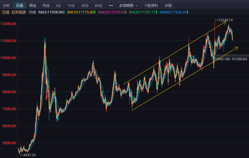
观察红利低波指数的走势可以观察到，红利低波指数近6年时间稳定地在一个上升通道区间内做震荡，因此希望利用这一点制定一个简单但收益率较高的策略，或许可以因此博取更高收益。

选择红利低波指数的原因，是因为其策略本身的优点。它选取50只流动性好，连续分红，红利支付率适中，每股股息正增长以及股息率高且波动率低的证券作为指数样本，采用股息率加权，反映分红水平高且波动率低的证券的整体表现。总体上说，红利低波可以保证10%左右的年化收益率，且波动幅度相对来说非常小。可以说红利低波指数是最适合大部分人的投资标的。

注意：本策略不具有普适性，历史数据不反映未来业绩，无任何投资建议，投资有风险，入市需谨慎。

策略雏形

本策略的雏形源自一种傻瓜式的网格定投法，即每跌4%就买入一成仓位，每涨4%就卖出1成仓位。这种策略的缺点在于资金利用率太低，再加上红利低波本身的波动就小，哪怕将阈值改为2%或者1%也并不能带来很好的收益率，且跑不赢满仓拿住不动。

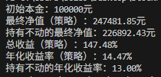
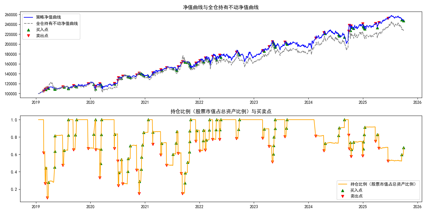
所以我针对参数进行优化，提出以下策略：价格每跌1%就买入2成仓，每涨5%就卖出4成仓。

通过写一段简短的Python代码，我们对数据进行简单的回测，以10万本金为例。可以得到如下结论：

代码如下：

# 固定金额网格
import pandas as pd
import matplotlib.pyplot as plt
import numpy as np# 设置中文字体
plt.rcParams['font.sans-serif'] = ['SimHei']  # 使用 SimHei 字体，支持中文
plt.rcParams['axes.unicode_minus'] = False  # 解决负号显示问题# 读取数据
data = pd.read_excel('512890.xlsx')
data['时间'] = pd.to_datetime(data['时间'])# 初始设置
initial_capital = 100000  # 初始本金
capital = initial_capital  # 当前资金
position = 0  # 当前持仓
cash = capital  # 可用现金
last_trade_price = None  # 上次交易价格
buy_threshold = -0.01  # 跌幅1%
sell_threshold = 0.05  # 涨幅5%
buy_amount = 20000  # 每次加仓2万元
sell_amount = 40000  # 每次卖出4万元# 保存数据用于计算收益
equity_curve = []  # 策略净值曲线
position_curve = []  # 持仓曲线（股票市值占总资产比例）
buy_sell_points = []  # 买卖点# 初始化全仓持有不动的净值曲线
buy_and_hold_equity_curve = [initial_capital]  # 初始全仓买入持有不动的净值# 模拟交易
for i, row in data.iterrows():close_price = row['收盘']# 如果是第一次交易，初始化并执行全仓买入if last_trade_price is None:position = initial_capital / close_price  # 全仓买入capital = 0  # 本金已经用完last_trade_price = close_priceequity_curve.append(initial_capital)  # 初始净值position_curve.append(position * close_price / initial_capital)  # 初始持仓比例（100%）continue# 判断是否需要加仓或卖出if close_price <= last_trade_price * (1 + buy_threshold):  # 跌幅1%# 加仓2万，检查是否有足够的现金if capital >= buy_amount:position += buy_amount / close_pricecapital -= buy_amountlast_trade_price = close_pricebuy_sell_points.append(('Buy', row['时间'], close_price))elif close_price >= last_trade_price * (1 + sell_threshold):  # 涨幅5%# 卖出4万，检查是否有足够的股票if position * close_price >= sell_amount:sell_value = min(sell_amount, position * close_price)position -= sell_value / close_pricecapital += sell_valuelast_trade_price = close_pricebuy_sell_points.append(('Sell', row['时间'], close_price))# 计算当前净值和持仓比例（股票市值占总资产的比例）current_value = capital + position * close_priceequity_curve.append(current_value)position_curve.append(position * close_price / current_value)  # 持仓比例# 计算全仓买入持有不动的净值曲线buy_and_hold_equity_curve.append(initial_capital * close_price / data['收盘'].iloc[0])# 计算年化收益率
days = (data['时间'].iloc[-1] - data['时间'].iloc[0]).days
total_return = (equity_curve[-1] - initial_capital) / initial_capital
annualized_return = (1 + total_return) ** (365 / days) - 1# 计算持有不动的年化收益率
buy_and_hold_total_return = (buy_and_hold_equity_curve[-1] - initial_capital) / initial_capital
buy_and_hold_annualized_return = (1 + buy_and_hold_total_return) ** (365 / days) - 1# 计算持有不动的最终净值
buy_and_hold_final_value = buy_and_hold_equity_curve[-1]# 输出收益指标
print(f"初始本金：{initial_capital}元")
print(f"最终净值（策略）：{equity_curve[-1]:.2f}元")
print(f"持有不动的最终净值：{buy_and_hold_final_value:.2f}元")
print(f"总收益（策略）：{total_return * 100:.2f}%")
print(f"年化收益率（策略）：{annualized_return * 100:.2f}%")
print(f"持有不动的年化收益率：{buy_and_hold_annualized_return * 100:.2f}%")# 绘制净值曲线、持仓比例曲线和买卖点
plt.figure(figsize=(14, 7))# 净值曲线（包含全仓持有不动的参考曲线）
plt.subplot(2, 1, 1)
plt.plot(data['时间'], equity_curve, label='策略净值曲线', color='blue')
plt.plot(data['时间'], buy_and_hold_equity_curve, label='全仓持有不动净值曲线', color='grey', linestyle='--')# 使用实际净值曲线的值来绘制买入卖出点
buy_prices = [point[2] for point in buy_sell_points if point[0] == 'Buy']
buy_times = [point[1] for point in buy_sell_points if point[0] == 'Buy']
sell_prices = [point[2] for point in buy_sell_points if point[0] == 'Sell']
sell_times = [point[1] for point in buy_sell_points if point[0] == 'Sell']# 获取买入卖出点的净值
buy_values = [equity_curve[data[data['时间'] == t].index[0]] for t in buy_times]
sell_values = [equity_curve[data[data['时间'] == t].index[0]] for t in sell_times]# 标出买入和卖出点
plt.scatter(buy_times, buy_values, marker='^', color='green', label='买入点')
plt.scatter(sell_times, sell_values, marker='v', color='red', label='卖出点')plt.legend()
plt.title('净值曲线与全仓持有不动净值曲线')# 绘制持仓比例曲线（股票市值占总资产的比例）
plt.subplot(2, 1, 2)
plt.plot(data['时间'], position_curve, label='持仓比例（股票市值占总资产比例）', color='orange')
plt.scatter(buy_times, [position_curve[data[data['时间'] == t].index[0]] for t in buy_times],marker='^', color='green', label='买入点')
plt.scatter(sell_times, [position_curve[data[data['时间'] == t].index[0]] for t in sell_times],marker='v', color='red', label='卖出点')
plt.legend()
plt.title('持仓比例（股票市值占总资产比例）与买卖点')plt.tight_layout()
plt.savefig('跌1%买2万 涨5%卖4万.png')
plt.show()

此策略仅仅带来不到1.5%的增幅，且经过我遍历大量的参数组合后发现，这种策略能够带来的收益上限也极其有限，我上面给出的策略几乎已经是表现最好的参数之一了。但是考虑到股票本身的不确定性，仅仅这点收益的增长完全可以归结于数据的偶然性，此策略本质上没有太大意义，无非就是在其中的一些时间段可以留出一部分本金，保证一定的流动性。

考虑优化

1.构建上升通道区间

接下来我们转变思路，既然水平的网格交易模式表现较差，那么是否可以构建一个上升式的通道区间，在区间内确定低点和高点，实现进阶网格交易？

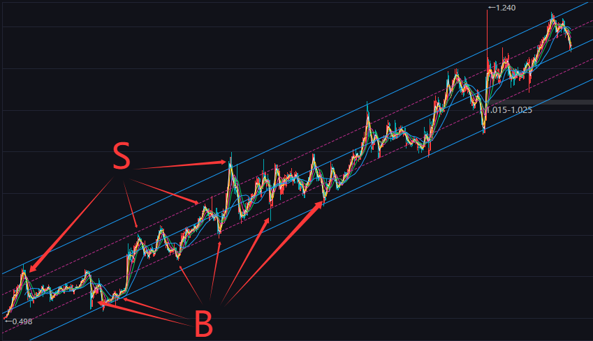
我的初步策略构想是这样的：在上升通道区间的低点分批建仓，在区间高点分批减仓。一个非常简单的逻辑，如下图所示。

具体到操作细节，我们这里暂定为：

首先构建三条平行线，上沿平行线用于描述价格波动的上限，下沿平行线描述价格波动的下限，中间线处于以上两根线的正中间，用于描述价格始终围绕中间线做上下波动。同时，再构造两根线，均平行于以上构造的三根线。这两根线其中一根处于上沿线与中线之间一半的位置，我称之为S线，另一根处于中线与下沿线之间一半的位置，我称之为B线。我策略如下：当价格下穿B线时，触发一次购买，默认买入65%的仓位，当继续下行至靠近下沿线时，再触发一次购买，这里默认是35%的仓位，也就是购买后已经满仓；相应地，当价格上穿S线时，卖出65%，当继续上行至靠近上沿线时，卖出剩下的35%。需要注意的是，如果价格只在B线触发了一次购买就回到了S线，那么这里卖出的量就是对应B线触发的买入的量。如果价格在B线反复波动，那么我们不会多次触发购买，只会触发一次，也就是说，如果最近一次购买是在B线处，那么下一次购买一定是继续下行到下沿线附近时触发，而不会是B线处连续两次的购买。 卖出同理，不会在S线处连续卖出。按以上的逻辑来讲，我们最多连续买两次，一次B线一次下沿线，最多也连续卖两次，一次S线一次上沿线。如果价格在S线和B线之间反复波动，那么我们的策略实际上就之会在B线买一次，S线卖一次，然后继续B线买S线卖。

---

通道线的计算方式如下：

1. 首先先用一元线性回归得到中线 mid
2. 计算每一天对中线的偏离：resid = price - mid
3. 取绝对偏离的分位数：w0 = np.quantile(|resid|, channel_quantile)
4. 把这个 w0（再经 width_scale/width_extra 调整）作为通道半宽 w，于是
   上沿 = mid + w
   下沿 = mid - w
   S/B 线也按 w 的比例定位

channel_quantile 这个参数用来决定通道的半宽度 w取多大。

如果设 channel_quantile = 0.90，那么 w 选的是“|resid| 的 90% 分位数”。这意味着大约90% 的价格会落在中线 ± w 的带内（极端点/离群点可能被排在外面）。

调大 channel_quantile → w 变宽 → 价格更不容易触发 B/S 线（信号更少、更稳）。

调小 channel_quantile → w 变窄 → 更容易触发（信号更多、更频繁）。

为什么用“分位数”而不是标准差？

因为分位数对离群点更鲁棒：一两次异常波动不会把通道拉得过宽。

越接近 1 的分位数，越接近“包含绝大多数样本”的宽度；越接近 0.5，通道会比较窄。

一般 0.85 ~ 0.95 比较常见；

---

另外，由于我们没有必要等价格真的完全突破区间上下沿线再执行买卖，只需要当价格靠近这条线附近时就可以触发。

我用以下参数来描述这种“靠近”：

near_upper_frac = 0.05          # “靠近上沿”的距离阈值（相对通道半宽的比例）
near_lower_frac = 0.1           # “靠近下沿”的距离阈值（相对通道半宽的比例）

2.确定买卖点

我用以下参数来确定BS线的位置：

s_pos = 0.5                     # S线在中线->上沿之间的位置比例 [0,1]
b_pos = 0.5                     # B线在中线->下沿之间的位置比例 [0,1]

并用以下参数来控制买卖的仓位：

buy_pct1 = 0.65                 # 第一次买入（B线触发）金额占当日总资产比例
buy_pct2 = 0.35                 # 第二次买入（靠近下沿触发）金额占当日总资产比例

3.测试收益率

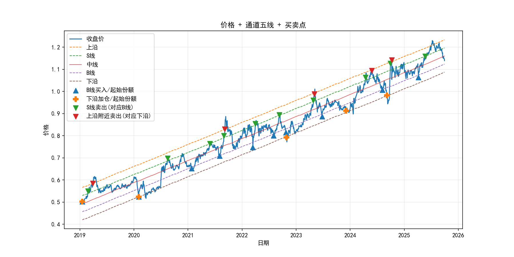
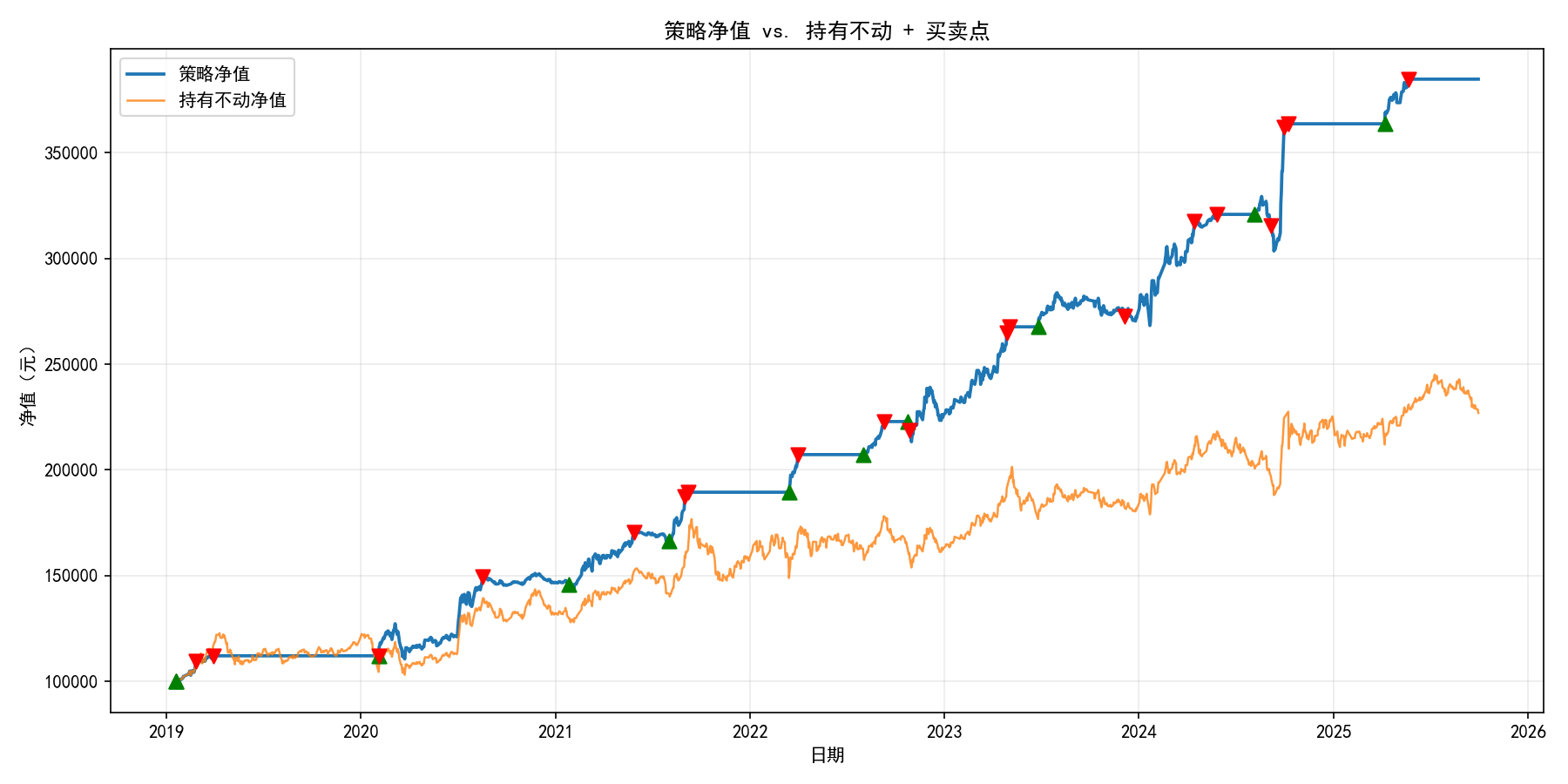
通过以上策略在过去6年多的时间进行复盘，我们可以得到如下结果：

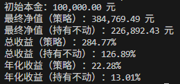
在接近7年的时间里，我们的策略让本金翻了接近3倍，达到了高达22.28%的年化收益率。具体的买卖点与净值曲线如下图所示。


代码如下：

# -*- coding: utf-8 -*-
import pandas as pd
import numpy as np
import matplotlib.pyplot as plt
from pathlib import Path# 通道波段策略
# ===================== 参数区（可按需调整） =====================
data_file = '512890.xlsx'       # 数据文件名（与脚本同目录）
initial_capital = 100000        # 初始现金（元）
fee_rate = 0.0                  # 单边手续费比例（默认0，可设 0.0005 等）channel_quantile = 0.90         # 通道宽度的分位数（残差 |e| 的分位数，默认90%），意味着大约90%的数据会落在分布带中。分位数对离群点更鲁棒：一两次异常波动不会把通道拉得过宽。
s_pos = 0.5                     # S线在中线->上沿之间的位置比例 [0,1]
b_pos = 0.5                     # B线在中线->下沿之间的位置比例 [0,1]
near_upper_frac = 0.05          # “靠近上沿”的距离阈值（相对通道半宽的比例）
near_lower_frac = 0.1           # “靠近下沿”的距离阈值（相对通道半宽的比例）# ★ 新增：通道宽度缩放（不改变中线位置）
width_scale = 1.1               # >1 放大间距，<1 缩小间距；默认1.0不改变
width_extra = 0.0               # 绝对增量（与价格同单位），默认0buy_pct1 = 0.65                 # 第一次买入（B线触发）金额占当日总资产比例
buy_pct2 = 0.35                 # 第二次买入（靠近下沿触发）金额占当日总资产比例
# 说明：卖出金额严格与相应买入的“那一笔”对应，不单独使用 sell_pct，
#      若你希望改为固定百分比卖出，可在下方“卖出逻辑”处按注释替换。# ★ 新增：是否在第一天默认全仓买入（用 buy_pct1 / buy_pct2 拆成两笔）
init_full_position = True# Matplotlib 中文与显示
plt.rcParams['font.sans-serif'] = ['SimHei', 'Microsoft YaHei', 'Arial Unicode MS']
plt.rcParams['axes.unicode_minus'] = False# ===================== 数据读取与列名识别 =====================
path = Path(data_file)
if not path.exists():raise FileNotFoundError(f'未找到数据文件：{data_file}（请与脚本放在同一目录）')df = pd.read_excel(path)# 识别日期列
date_cols_try = ['时间', '日期', '交易日期', 'Date', 'date', '交易日']
date_col = None
for c in date_cols_try:if c in df.columns:date_col = cbreak
if date_col is None:raise ValueError('未识别到日期列（例如：时间/日期/交易日期/Date）。请检查数据列名。')df[date_col] = pd.to_datetime(df[date_col])
df = df.sort_values(by=date_col).reset_index(drop=True)# 识别收盘价列
close_cols_try = ['收盘', '收盘价', '收盘价(元)', 'Close', 'close', '收盘价（元）']
close_col = None
for c in close_cols_try:if c in df.columns:close_col = cbreak
if close_col is None:numeric_cols = [c for c in df.columns if c != date_col and pd.api.types.is_numeric_dtype(df[c])]if not numeric_cols:raise ValueError('未识别到收盘价列（例如：收盘/收盘价/Close）。请检查数据列名。')close_col = numeric_cols[-1]prices = df[close_col].astype(float).values
dates = df[date_col].values
n = len(prices)
if n < 3:raise ValueError('数据量太少，无法构建通道。')# ===================== 构建通道（上沿/中线/下沿 + S/B） =====================
x = np.arange(n).astype(float)
b, a = np.polyfit(x, prices, 1)  # [斜率, 截距]
mid = a + b * xresid = prices - mid
w0 = np.quantile(np.abs(resid), channel_quantile)
min_w = 0.005 * np.median(prices)
w0 = max(w0, min_w)
w = max(w0 * width_scale + width_extra, min_w)upper = mid + w
lower = mid - w
S_line = mid + s_pos * w
B_line = mid - b_pos * wnear_upper_dist = near_upper_frac * w
near_lower_dist = near_lower_frac * w# ===================== 策略回测（状态机+两笔分批） =====================
cash = float(initial_capital)
shares = 0.0# 分笔持仓：b_lot 对应 B线买入；l_lot 对应“靠近下沿”买入
b_lot_qty = 0.0
l_lot_qty = 0.0equity_curve = []
bh_equity_curve = []# 基准：第一天全仓买入并持有
first_price = prices[0]
bh_shares = initial_capital / first_price# 交易记录
trades = []  # dict: time, price, action, qty, cash_delta, shares_after, equitydef total_equity(p):return cash + shares * p# ★★★ 起始建仓：第一天默认全仓买入（拆成两笔，对应后续 S/上沿 的卖出）
if init_full_position:p0 = first_priceequity0 = initial_capital# 第一笔：B线份额buy_cash1 = min(equity0 * buy_pct1, cash)if buy_cash1 > 1e-8 and p0 > 0:qty1 = buy_cash1 * (1 - fee_rate) / p0cash -= buy_cash1shares += qty1b_lot_qty += qty1trades.append({'time': dates[0], 'price': p0, 'action': '起始建仓(B线份额)','qty': qty1, 'cash_delta': -buy_cash1,'shares_after': shares, 'equity': total_equity(p0)})# 第二笔：下沿份额buy_cash2 = min(equity0 * buy_pct2, cash)  # 用起始总资产拆分，保证买_pct 之和=1时为满仓if buy_cash2 > 1e-8 and p0 > 0:qty2 = buy_cash2 * (1 - fee_rate) / p0cash -= buy_cash2shares += qty2l_lot_qty += qty2trades.append({'time': dates[0], 'price': p0, 'action': '起始建仓(下沿份额)','qty': qty2, 'cash_delta': -buy_cash2,'shares_after': shares, 'equity': total_equity(p0)})# 若 buy_pct1 + buy_pct2 < 1，保留未用现金；>1 则第二笔按剩余现金自动截断prev_p = prices[0]
prev_B = B_line[0]
prev_S = S_line[0]for i in range(n):p = prices[i]# 基准净值bh_equity_curve.append(bh_shares * p)# —— 卖出侧 ——（先处理）if i > 0:# 上穿 S：卖出“B线那一笔”if (prev_p < prev_S) and (p >= S_line[i]):if b_lot_qty > 0:sell_qty = min(b_lot_qty, shares)if sell_qty > 1e-12:proceeds = sell_qty * p * (1 - fee_rate)cash += proceedsshares -= sell_qtyb_lot_qty -= sell_qtytrades.append({'time': dates[i], 'price': p, 'action': 'S线卖出(对应B线)','qty': -sell_qty, 'cash_delta': proceeds,'shares_after': shares, 'equity': total_equity(p)})# 触及上沿附近：卖出“下沿那一笔”if l_lot_qty > 0:if p >= (upper[i] - near_upper_dist):sell_qty = min(l_lot_qty, shares)if sell_qty > 1e-12:proceeds = sell_qty * p * (1 - fee_rate)cash += proceedsshares -= sell_qtyl_lot_qty -= sell_qtytrades.append({'time': dates[i], 'price': p, 'action': '上沿附近卖出(对应下沿加仓)','qty': -sell_qty, 'cash_delta': proceeds,'shares_after': shares, 'equity': total_equity(p)})# —— 买入侧 ——# 下穿 B：若尚无 B 线那一笔，则买入if i > 0:if (prev_p > prev_B) and (p <= B_line[i]):if b_lot_qty <= 1e-12:target_cash = total_equity(p) * buy_pct1buy_cash = min(target_cash, cash)if buy_cash > 1e-8 and p > 0:qty = buy_cash * (1 - fee_rate) / pcash -= buy_cashshares += qtyb_lot_qty += qtytrades.append({'time': dates[i], 'price': p, 'action': 'B线买入','qty': qty, 'cash_delta': -buy_cash,'shares_after': shares, 'equity': total_equity(p)})# 触及下沿附近：若已有 B 线那一笔且尚无下沿那一笔，则再买if (b_lot_qty > 1e-12) and (l_lot_qty <= 1e-12):if p <= (lower[i] + near_lower_dist):target_cash = total_equity(p) * buy_pct2buy_cash = min(target_cash, cash)if buy_cash > 1e-8 and p > 0:qty = buy_cash * (1 - fee_rate) / pcash -= buy_cashshares += qtyl_lot_qty += qtytrades.append({'time': dates[i], 'price': p, 'action': '下沿附近加仓','qty': qty, 'cash_delta': -buy_cash,'shares_after': shares, 'equity': total_equity(p)})# 记录每日策略净值equity_curve.append(total_equity(p))prev_p = pprev_B = B_line[i]prev_S = S_line[i]equity_curve = np.array(equity_curve, dtype=float)
bh_equity_curve = np.array(bh_equity_curve, dtype=float)# ===================== 绩效统计 =====================
final_equity = float(equity_curve[-1])
final_bh = float(bh_equity_curve[-1])total_return = final_equity / initial_capital - 1.0
bh_return = final_bh / initial_capital - 1.0days = (pd.to_datetime(dates[-1]) - pd.to_datetime(dates[0])).days
years = days / 365.25 if days > 0 else 0
def ann_ret(v0, v1, yrs):if yrs <= 0 or v0 <= 0:return np.nanreturn (v1 / v0) ** (1.0 / yrs) - 1.0ann_return = ann_ret(initial_capital, final_equity, years)
bh_ann_return = ann_ret(initial_capital, final_bh, years)print(f'初始本金：{initial_capital:,.2f} 元')
print(f'最终净值（策略）：{final_equity:,.2f} 元')
print(f'最终净值（持有不动）：{final_bh:,.2f} 元')
print(f'总收益（策略）：{total_return*100:.2f}%')
print(f'总收益（持有不动）：{bh_return*100:.2f}%')
if not np.isnan(ann_return):print(f'年化收益（策略）：{ann_return*100:.2f}%')
if not np.isnan(bh_ann_return):print(f'年化收益（持有不动）：{bh_ann_return*100:.2f}%')# ===================== 画图 =====================
# 1) 价格 + 通道五线 + 买卖点
fig1, ax1 = plt.subplots(figsize=(12, 6))
ax1.plot(dates, prices, label='收盘价', linewidth=1.5)
ax1.plot(dates, upper, '--', label='上沿', linewidth=1.0)
ax1.plot(dates, S_line, '--', label='S线', linewidth=1.0)
ax1.plot(dates, mid, '-', label='中线', linewidth=1.0, alpha=0.7)
ax1.plot(dates, B_line, '--', label='B线', linewidth=1.0)
ax1.plot(dates, lower, '--', label='下沿', linewidth=1.0)# 标注买卖点（价格图）
if len(trades) > 0:buy_B_x = [t['time'] for t in trades if 'B线买入' in t['action'] or '起始建仓(B线份额)' in t['action']]buy_B_y = [t['price'] for t in trades if 'B线买入' in t['action'] or '起始建仓(B线份额)' in t['action']]buy_L_x = [t['time'] for t in trades if '下沿附近加仓' in t['action'] or '起始建仓(下沿份额)' in t['action']]buy_L_y = [t['price'] for t in trades if '下沿附近加仓' in t['action'] or '起始建仓(下沿份额)' in t['action']]sell_S_x = [t['time'] for t in trades if 'S线卖出' in t['action']]sell_S_y = [t['price'] for t in trades if 'S线卖出' in t['action']]sell_U_x = [t['time'] for t in trades if '上沿附近卖出' in t['action']]sell_U_y = [t['price'] for t in trades if '上沿附近卖出' in t['action']]ax1.scatter(buy_B_x, buy_B_y, marker='^', s=70, label='B线买入/起始份额', zorder=5)ax1.scatter(buy_L_x, buy_L_y, marker='P', s=70, label='下沿加仓/起始份额', zorder=5)ax1.scatter(sell_S_x, sell_S_y, marker='v', s=70, label='S线卖出(对应B线)', zorder=5)ax1.scatter(sell_U_x, sell_U_y, marker='v', s=70, label='上沿附近卖出(对应下沿)', zorder=5)ax1.set_title('价格 + 通道五线 + 买卖点')
ax1.set_xlabel('日期')
ax1.set_ylabel('价格')
ax1.legend(loc='best')
ax1.grid(alpha=0.25)# 2) 净值曲线 + 买卖点
fig2, ax2 = plt.subplots(figsize=(12, 6))
ax2.plot(dates, equity_curve, label='策略净值', linewidth=1.8)
ax2.plot(dates, bh_equity_curve, label='持有不动净值', linewidth=1.2, alpha=0.8)# 在净值图上也标注买卖点（用当日策略净值）
if len(trades) > 0:bx = [t['time'] for t in trades]by = [t['equity'] for t in trades]colors = []markers = []for t in trades:if '买入' in t['action'] or '起始建仓' in t['action']:colors.append('green'); markers.append('^')else:colors.append('red'); markers.append('v')for x_i, y_i, m_i, c_i in zip(bx, by, markers, colors):ax2.scatter(x_i, y_i, marker=m_i, s=60, color=c_i, zorder=5)ax2.set_title('策略净值 vs. 持有不动 + 买卖点')
ax2.set_xlabel('日期')
ax2.set_ylabel('净值（元）')
ax2.legend(loc='best')
ax2.grid(alpha=0.25)plt.tight_layout()
plt.show()
# 如需保存图片，建议放在 plt.show() 之前（避免某些环境下空图）：
fig1.savefig('价格_通道_买卖点.png', dpi=150)
fig2.savefig('净值曲线_买卖点.png', dpi=150)# ===================== 使用说明与可选改动 =====================
# 1) 若你希望“卖出比例可独立设置”，而不是严格对应那一笔买入，
#    可以把“卖出逻辑”里 sell_qty 的定义替换为：
#      - S线卖出：sell_qty = min(shares, (total_equity(p) * sell_pct1) / p)
#      - 上沿卖出：sell_qty = min(shares, (total_equity(p) * sell_pct2) / p)
#    并在参数区添加 sell_pct1、sell_pct2（默认 0.5）。
#
# 2) 通道宽度：当前使用 |残差| 的分位数（channel_quantile）来控制包含度；
#    或改为 k 倍标准差：w = k * resid.std()。
#
# 3) “靠近上/下沿”的定义：使用 near_upper_frac/near_lower_frac * w 的距离阈值。
#
# 4) 资金使用：买入金额以“当日总资产”为基准，自动受“现金余额”约束；卖出按对应分笔数量。
#    起始建仓后，会先等待卖出触发；当两笔都卖完后，才会进入下一轮 B/下沿 的买入。
#
# 注意：代码的线（中线/通道宽度）是用到今天为止的历史重新估出来的，所以每天的阈值会随数据滚动更新（这在实盘里是合理的“当期可见信息”）。

4.优化参数组合

考虑到我们当前敲定的参数组合可能并不是最优解，因此我们需要搜索更优的参数组合。

这里我使用小网格搜索 + 走步验证（walk-forward）+ 指标表的方式，在前 60% 样本做调参（训练集），在后 40% 做验证（测试集），输出每个参数组合在训练/测试上的 CAGR复合年化、总收益、最大回撤、Sharpe夏普比率、交易次数。

运行后我们得到如下结果：

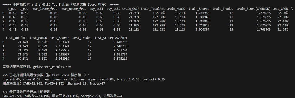
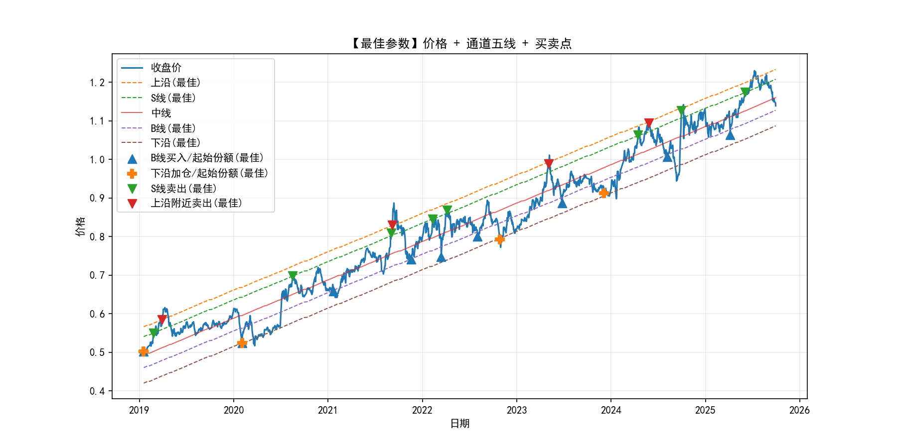
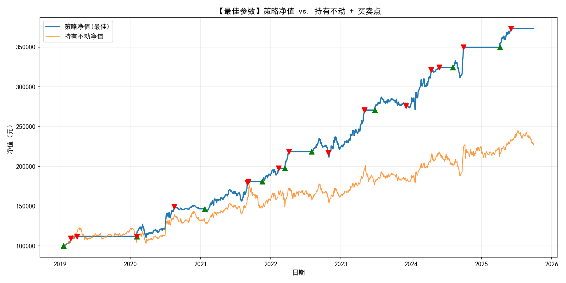
通过此方法搜索到的最佳参数组合为：

设置B线在35%的位置，S线在65%的位置，下沿线“靠近阈值”为10%，上沿线“靠近阈值”为5%，B线买入仓位为65%，下沿线买入仓位为35%

在测试集上的表现为：CAGR年化=21.72%, 总收益=273.19%, 最大回撤=13.11%, Sharpe夏普比率=1.93, 交易次数=24
从夏普比率来看，此策略的风险收益比相当优秀。

（需要注意的是，这一步的收益率没有上一章节高，原因是这里将原始数据划分为训练集和测试集了，得出的收益率是测试集上的数据，所以会有一定的差距，但这也侧面说明此策略具有一定的健壮性）

具体情况如下图：


代码如下：

# -*- coding: utf-8 -*-
import pandas as pd
import numpy as np
import matplotlib.pyplot as plt
from pathlib import Path# ===================== 参数区（可按需调整） =====================
data_file = '512890.xlsx'       # 数据文件名（与脚本同目录）
initial_capital = 100000        # 初始现金（元）
fee_rate = 0.0                  # 单边手续费比例（默认0，可设 0.0005 等）channel_quantile = 0.90         # 通道宽度分位数（|残差|的分位数）
s_pos = 0.5                     # S线在中线->上沿之间的位置比例 [0,1]
b_pos = 0.5                     # B线在中线->下沿之间的位置比例 [0,1]
near_upper_frac = 0.05          # “靠近上沿”的阈值（相对半宽比例）
near_lower_frac = 0.10          # “靠近下沿”的阈值（相对半宽比例）# 通道宽度缩放（不改变中线）
width_scale = 1.1               # >1 放大间距，<1 缩小间距
width_extra = 0.0               # 绝对增量（与价格同单位）# 仓位分配
buy_pct1 = 0.65                 # 第一次买入（B线触发）金额占当日总资产比例
buy_pct2 = 0.35                 # 第二次买入（下沿附近触发）金额占当日总资产比例# 第一日起始建仓
init_full_position = True       # True：第一天按 buy_pct1/buy_pct2 拆成两笔建仓# ====== 网格搜索与走步验证设置 ======
do_grid_search = True           # 是否执行小网格搜索 + 走步验证
train_ratio = 0.60              # 训练/验证划分（按时间顺序）
# 小网格（先定“时点”）：B/S 位置 + 上/下沿触发距离
grid_b_pos = [0.45, 0.55, 0.65]
grid_s_pos = [0.55, 0.65, 0.75]
grid_near_lower = [0.10, 0.15]
grid_near_upper = [0.05, 0.10]
# 可选：第二步微调仓位（默认关闭，避免计算太多）
enable_buy_grid = False
grid_buy_pct1 = [max(0.2, buy_pct1-0.1), buy_pct1, min(0.8, buy_pct1+0.1)]
grid_buy_pct2 = [max(0.2, buy_pct2-0.1), buy_pct2, min(0.8, buy_pct2+0.1)]# Matplotlib 中文与显示
plt.rcParams['font.sans-serif'] = ['SimHei', 'Microsoft YaHei', 'Arial Unicode MS']
plt.rcParams['axes.unicode_minus'] = False# ===================== 数据读取与列名识别 =====================
path = Path(data_file)
if not path.exists():raise FileNotFoundError(f'未找到数据文件：{data_file}（请与脚本放在同一目录）')df = pd.read_excel(path)# 识别日期列
date_cols_try = ['时间', '日期', '交易日期', 'Date', 'date', '交易日']
date_col = None
for c in date_cols_try:if c in df.columns:date_col = cbreak
if date_col is None:raise ValueError('未识别到日期列（例如：时间/日期/交易日期/Date）。请检查数据列名。')df[date_col] = pd.to_datetime(df[date_col])
df = df.sort_values(by=date_col).reset_index(drop=True)# 识别收盘价列
close_cols_try = ['收盘', '收盘价', '收盘价(元)', 'Close', 'close', '收盘价（元）']
close_col = None
for c in close_cols_try:if c in df.columns:close_col = cbreak
if close_col is None:numeric_cols = [c for c in df.columns if c != date_col and pd.api.types.is_numeric_dtype(df[c])]if not numeric_cols:raise ValueError('未识别到收盘价列（例如：收盘/收盘价/Close）。请检查数据列名。')close_col = numeric_cols[-1]prices = df[close_col].astype(float).values
dates = df[date_col].values
n = len(prices)
if n < 50:raise ValueError('样本太少，建议至少 50 根K线。')# ===================== 通用函数 =====================
def build_channel(prices_local, channel_quantile, width_scale, width_extra, s_pos, b_pos,near_upper_frac, near_lower_frac):"""基于当前窗口数据构建通道五线与触发距离"""m = len(prices_local)x = np.arange(m).astype(float)slope, intercept = np.polyfit(x, prices_local, 1)  # [斜率, 截距]mid = intercept + slope * xresid = prices_local - midw0 = np.quantile(np.abs(resid), channel_quantile)min_w = 0.005 * np.median(prices_local)            # 至少中位价的0.5%w0 = max(w0, min_w)w = max(w0 * width_scale + width_extra, min_w)upper = mid + wlower = mid - wS_line = mid + s_pos * wB_line = mid - b_pos * wnear_upper_dist = near_upper_frac * wnear_lower_dist = near_lower_frac * wreturn mid, upper, lower, S_line, B_line, near_upper_dist, near_lower_distdef backtest_once(prices_local, dates_local, params):"""按给定参数在一个窗口内回测，返回指标、净值曲线、交易记录"""(channel_quantile, width_scale, width_extra, s_pos, b_pos,near_upper_frac, near_lower_frac, buy_pct1, buy_pct2,fee_rate, init_full_position) = paramsmid, upper, lower, S_line, B_line, near_U, near_L = build_channel(prices_local, channel_quantile, width_scale, width_extra, s_pos, b_pos,near_upper_frac, near_lower_frac)cash = float(initial_capital)shares = 0.0b_lot_qty = 0.0l_lot_qty = 0.0equity_curve = []trades = []# 基准：第一天全仓买入（买入持有）first_price = prices_local[0]bh_shares = initial_capital / first_pricebh_equity_curve = [bh_shares * p for p in prices_local]def total_equity(p): return cash + shares * p# 起始建仓（按两笔拆分）if init_full_position:p0 = first_priceeq0 = initial_capital# B线份额buy_cash1 = min(eq0 * buy_pct1, cash)if buy_cash1 > 1e-8 and p0 > 0:qty1 = buy_cash1 * (1 - fee_rate) / p0cash -= buy_cash1; shares += qty1; b_lot_qty += qty1trades.append({'time': dates_local[0], 'price': p0, 'action': '起始建仓(B线份额)','qty': qty1, 'cash_delta': -buy_cash1,'shares_after': shares, 'equity': total_equity(p0)})# 下沿份额buy_cash2 = min(eq0 * buy_pct2, cash)if buy_cash2 > 1e-8 and p0 > 0:qty2 = buy_cash2 * (1 - fee_rate) / p0cash -= buy_cash2; shares += qty2; l_lot_qty += qty2trades.append({'time': dates_local[0], 'price': p0, 'action': '起始建仓(下沿份额)','qty': qty2, 'cash_delta': -buy_cash2,'shares_after': shares, 'equity': total_equity(p0)})prev_p = prices_local[0]prev_B = B_line[0]prev_S = S_line[0]for i, p in enumerate(prices_local):# —— 卖出侧 —— 先处理if i > 0:# 上穿 S：卖出“B线那一笔”if (prev_p < prev_S) and (p >= S_line[i]):if b_lot_qty > 0:sell_qty = min(b_lot_qty, shares)if sell_qty > 1e-12:proceeds = sell_qty * p * (1 - fee_rate)cash += proceeds; shares -= sell_qty; b_lot_qty -= sell_qtytrades.append({'time': dates_local[i], 'price': p, 'action': 'S线卖出(对应B线)','qty': -sell_qty, 'cash_delta': proceeds,'shares_after': shares, 'equity': total_equity(p)})# 上沿附近：卖出“下沿那一笔”if l_lot_qty > 0 and p >= (upper[i] - near_U):sell_qty = min(l_lot_qty, shares)if sell_qty > 1e-12:proceeds = sell_qty * p * (1 - fee_rate)cash += proceeds; shares -= sell_qty; l_lot_qty -= sell_qtytrades.append({'time': dates_local[i], 'price': p, 'action': '上沿附近卖出(对应下沿)','qty': -sell_qty, 'cash_delta': proceeds,'shares_after': shares, 'equity': total_equity(p)})# —— 买入侧 ——if i > 0 and (prev_p > prev_B) and (p <= B_line[i]) and (b_lot_qty <= 1e-12):buy_cash = min(total_equity(p) * buy_pct1, cash)if buy_cash > 1e-8 and p > 0:qty = buy_cash * (1 - fee_rate) / pcash -= buy_cash; shares += qty; b_lot_qty += qtytrades.append({'time': dates_local[i], 'price': p, 'action': 'B线买入','qty': qty, 'cash_delta': -buy_cash,'shares_after': shares, 'equity': total_equity(p)})if (b_lot_qty > 1e-12) and (l_lot_qty <= 1e-12) and (p <= (lower[i] + near_L)):buy_cash = min(total_equity(p) * buy_pct2, cash)if buy_cash > 1e-8 and p > 0:qty = buy_cash * (1 - fee_rate) / pcash -= buy_cash; shares += qty; l_lot_qty += qtytrades.append({'time': dates_local[i], 'price': p, 'action': '下沿附近加仓','qty': qty, 'cash_delta': -buy_cash,'shares_after': shares, 'equity': total_equity(p)})equity_curve.append(total_equity(p))prev_p = p; prev_B = B_line[i]; prev_S = S_line[i]equity_curve = np.array(equity_curve, dtype=float)bh_equity_curve = np.array(bh_equity_curve, dtype=float)# 指标final_equity = float(equity_curve[-1])total_return = final_equity / initial_capital - 1.0days = (pd.to_datetime(dates_local[-1]) - pd.to_datetime(dates_local[0])).daysyears = days / 365.25 if days > 0 else np.nanCAGR = (final_equity / initial_capital) ** (1/years) - 1 if years and years > 0 else np.nan# 最大回撤peak = np.maximum.accumulate(equity_curve)dd = (equity_curve - peak) / peakmaxDD = -dd.min() if len(dd) > 0 else np.nan# Sharpe（按交易日 252）daily_ret = pd.Series(equity_curve).pct_change().dropna()if not daily_ret.empty:sharpe = np.sqrt(252) * daily_ret.mean() / (daily_ret.std(ddof=0) + 1e-12)else:sharpe = np.nan# 统计交易次数（不含起始建仓）trade_count = sum(1 for t in trades if '起始建仓' not in t['action'])metrics = {'CAGR': CAGR, 'TotalRet': total_return, 'MaxDD': maxDD, 'Sharpe': sharpe,'Trades': trade_count, 'EquityCurve': equity_curve, 'BHCurve': bh_equity_curve,'TradesList': trades}return metricsdef fmt_pct(x):return None if pd.isna(x) else f"{x*100:.2f}%"# ===================== 主回测（用当前参数绘图） =====================
# 先跑一遍主参数，便于可视化
params_main = (channel_quantile, width_scale, width_extra, s_pos, b_pos,near_upper_frac, near_lower_frac, buy_pct1, buy_pct2,fee_rate, init_full_position)
m_main = backtest_once(prices, dates, params_main)print(f'初始本金：{initial_capital:,.2f} 元')
print(f'最终净值（策略）：{m_main["EquityCurve"][-1]:,.2f} 元')
print(f'总收益（策略）：{fmt_pct(m_main["TotalRet"])}')
print(f'年化收益（策略）：{fmt_pct(m_main["CAGR"])}')
print(f'最大回撤（策略）：{fmt_pct(m_main["MaxDD"])}')
print(f'Sharpe（策略）：{m_main["Sharpe"]:.2f}')
print(f'交易次数：{m_main["Trades"]}')# ===== 画图：价格 + 五线 + 买卖点（用主参数重算通道） =====
mid, upper, lower, S_line_draw, B_line_draw, near_U_d, near_L_d = build_channel(prices, channel_quantile, width_scale, width_extra, s_pos, b_pos,near_upper_frac, near_lower_frac
)fig1, ax1 = plt.subplots(figsize=(12, 6))
ax1.plot(dates, prices, label='收盘价', linewidth=1.5)
ax1.plot(dates, upper, '--', label='上沿', linewidth=1.0)
ax1.plot(dates, S_line_draw, '--', label='S线', linewidth=1.0)
ax1.plot(dates, mid, '-', label='中线', linewidth=1.0, alpha=0.7)
ax1.plot(dates, B_line_draw, '--', label='B线', linewidth=1.0)
ax1.plot(dates, lower, '--', label='下沿', linewidth=1.0)trades_main = m_main['TradesList']
if len(trades_main) > 0:buy_B_x = [t['time'] for t in trades_main if 'B线买入' in t['action'] or '起始建仓(B线份额)' in t['action']]buy_B_y = [t['price'] for t in trades_main if 'B线买入' in t['action'] or '起始建仓(B线份额)' in t['action']]buy_L_x = [t['time'] for t in trades_main if '下沿附近加仓' in t['action'] or '起始建仓(下沿份额)' in t['action']]buy_L_y = [t['price'] for t in trades_main if '下沿附近加仓' in t['action'] or '起始建仓(下沿份额)' in t['action']]sell_S_x = [t['time'] for t in trades_main if 'S线卖出' in t['action']]sell_S_y = [t['price'] for t in trades_main if 'S线卖出' in t['action']]sell_U_x = [t['time'] for t in trades_main if '上沿附近卖出' in t['action']]sell_U_y = [t['price'] for t in trades_main if '上沿附近卖出' in t['action']]ax1.scatter(buy_B_x, buy_B_y, marker='^', s=70, label='B线买入/起始份额', zorder=5)ax1.scatter(buy_L_x, buy_L_y, marker='P', s=70, label='下沿加仓/起始份额', zorder=5)ax1.scatter(sell_S_x, sell_S_y, marker='v', s=70, label='S线卖出(对应B线)', zorder=5)ax1.scatter(sell_U_x, sell_U_y, marker='v', s=70, label='上沿附近卖出(对应下沿)', zorder=5)ax1.set_title('价格 + 通道五线 + 买卖点')
ax1.set_xlabel('日期'); ax1.set_ylabel('价格'); ax1.legend(loc='best'); ax1.grid(alpha=0.25)# 净值曲线
fig2, ax2 = plt.subplots(figsize=(12, 6))
ax2.plot(dates, m_main['EquityCurve'], label='策略净值', linewidth=1.8)
bh_curve = (initial_capital / prices[0]) * prices  # 买入持有
ax2.plot(dates, bh_curve, label='持有不动净值', linewidth=1.2, alpha=0.8)
if len(trades_main) > 0:bx = [t['time'] for t in trades_main]by = [t['equity'] for t in trades_main]for t, x_i, y_i in zip(trades_main, bx, by):mkr = '^' if ('买入' in t['action'] or '起始建仓' in t['action']) else 'v'col = 'green' if mkr == '^' else 'red'ax2.scatter(x_i, y_i, marker=mkr, s=60, color=col, zorder=5)
ax2.set_title('策略净值 vs. 持有不动 + 买卖点')
ax2.set_xlabel('日期'); ax2.set_ylabel('净值（元）'); ax2.legend(loc='best'); ax2.grid(alpha=0.25)plt.tight_layout()
# 如需保存图片，建议放在 show 之前
# fig1.savefig('价格_通道_买卖点.png', dpi=150)
# fig2.savefig('净值曲线_买卖点.png', dpi=150)
plt.show()# ===================== 小网格搜索 + 走步验证 =====================
if do_grid_search:split_idx = int(len(prices) * train_ratio)prices_train, dates_train = prices[:split_idx], dates[:split_idx]prices_test,  dates_test  = prices[split_idx:], dates[split_idx:]rows = []# 组装网格if enable_buy_grid:buy1_list = grid_buy_pct1buy2_list = grid_buy_pct2else:buy1_list = [buy_pct1]buy2_list = [buy_pct2]for bp in grid_b_pos:for sp in grid_s_pos:for nl in grid_near_lower:for nu in grid_near_upper:for b1 in buy1_list:for b2 in buy2_list:params_train = (channel_quantile, width_scale, width_extra,sp, bp, nu, nl, b1, b2, fee_rate, init_full_position)m_tr = backtest_once(prices_train, dates_train, params_train)score_tr = (m_tr['CAGR'] / max(m_tr['MaxDD'], 1e-6)if (m_tr['CAGR'] is not None and not pd.isna(m_tr['CAGR'])) else -np.inf)# 在测试集复用同一组参数独立回测（注意：每个窗口内部都会重新拟合通道）m_te = backtest_once(prices_test, dates_test, params_train)score_te = (m_te['CAGR'] / max(m_te['MaxDD'], 1e-6)if (m_te['CAGR'] is not None and not pd.isna(m_te['CAGR'])) else -np.inf)rows.append({'b_pos': bp, 's_pos': sp,'near_lower_frac': nl, 'near_upper_frac': nu,'buy_pct1': b1, 'buy_pct2': b2,'train_CAGR': m_tr['CAGR'], 'train_TotalRet': m_tr['TotalRet'],'train_MaxDD': m_tr['MaxDD'], 'train_Sharpe': m_tr['Sharpe'],'train_Trades': m_tr['Trades'], 'train_Score(CAGR/DD)': score_tr,'test_CAGR': m_te['CAGR'], 'test_TotalRet': m_te['TotalRet'],'test_MaxDD': m_te['MaxDD'], 'test_Sharpe': m_te['Sharpe'],'test_Trades': m_te['Trades'], 'test_Score(CAGR/DD)': score_te})res_df = pd.DataFrame(rows)# 排序：按测试集评分，其次按测试CAGRres_df_sorted = res_df.sort_values(by=['test_Score(CAGR/DD)', 'test_CAGR'], ascending=[False, False]).reset_index(drop=True)# 保存全量结果res_df_sorted.to_csv('gridsearch_results.csv', index=False, encoding='utf-8-sig')# 展示 Top-5（格式化输出）top5 = res_df_sorted.head(5).copy()def _fmt(df, cols_pct):for c in cols_pct:df[c] = df[c].apply(lambda x: fmt_pct(x) if pd.notna(x) else None)return dftop5_display = top5.copy()top5_display = _fmt(top5_display, ['train_CAGR','train_TotalRet','train_MaxDD','test_CAGR','test_TotalRet','test_MaxDD'])# 打印print('\n===== 小网格搜索 + 走步验证：Top-5 组合（按测试集 Score 排序） =====')with pd.option_context('display.max_columns', None, 'display.width', 180):print(top5_display[['b_pos','s_pos','near_lower_frac','near_upper_frac','buy_pct1','buy_pct2','train_CAGR','train_TotalRet','train_MaxDD','train_Sharpe','train_Trades','train_Score(CAGR/DD)','test_CAGR','test_TotalRet','test_MaxDD','test_Sharpe','test_Trades','test_Score(CAGR/DD)']])print('\n完整结果已保存到：gridsearch_results.csv')# —— 自动选取测试集最优参数并回填到主图，重新在全样本上回测与作图 —— #if not res_df_sorted.empty:best_row = res_df_sorted.iloc[0]# 打印最优参数与测试集成绩print('\n>>> 已选择测试集最优参数（按 test_Score 排序第一）：')print(f"b_pos={best_row['b_pos']}, s_pos={best_row['s_pos']}, "f"near_lower_frac={best_row['near_lower_frac']}, near_upper_frac={best_row['near_upper_frac']}, "f"buy_pct1={best_row['buy_pct1']}, buy_pct2={best_row['buy_pct2']}")print(f"测试集表现：CAGR={fmt_pct(best_row['test_CAGR'])}, "f"MaxDD={fmt_pct(best_row['test_MaxDD'])}, Sharpe={best_row['test_Sharpe']:.2f}, "f"Trades={int(best_row['test_Trades'])}")# 回填参数并在“全样本”上重跑一次best_params = (channel_quantile, width_scale, width_extra,float(best_row['s_pos']), float(best_row['b_pos']),float(best_row['near_upper_frac']), float(best_row['near_lower_frac']),float(best_row['buy_pct1']), float(best_row['buy_pct2']),fee_rate, init_full_position)m_best = backtest_once(prices, dates, best_params)# 再计算一遍五条线用于绘图（全样本 + 最优参数）mid_b, upper_b, lower_b, S_b, B_b, nearU_b, nearL_b = build_channel(prices, channel_quantile, width_scale, width_extra,float(best_row['s_pos']), float(best_row['b_pos']),float(best_row['near_upper_frac']), float(best_row['near_lower_frac']))# —— 图3：价格 + 五线 +（最优参数下的）买卖点 —— #fig3, ax3 = plt.subplots(figsize=(12, 6))ax3.plot(dates, prices, label='收盘价', linewidth=1.5)ax3.plot(dates, upper_b, '--', label='上沿(最佳)', linewidth=1.0)ax3.plot(dates, S_b, '--', label='S线(最佳)', linewidth=1.0)ax3.plot(dates, mid_b, '-', label='中线', linewidth=1.0, alpha=0.7)ax3.plot(dates, B_b, '--', label='B线(最佳)', linewidth=1.0)ax3.plot(dates, lower_b, '--', label='下沿(最佳)', linewidth=1.0)trades_best = m_best['TradesList']if len(trades_best) > 0:buy_B_x = [t['time'] for t in trades_best if 'B线买入' in t['action'] or '起始建仓(B线份额)' in t['action']]buy_B_y = [t['price'] for t in trades_best if 'B线买入' in t['action'] or '起始建仓(B线份额)' in t['action']]buy_L_x = [t['time'] for t in trades_best if '下沿附近加仓' in t['action'] or '起始建仓(下沿份额)' in t['action']]buy_L_y = [t['price'] for t in trades_best if '下沿附近加仓' in t['action'] or '起始建仓(下沿份额)' in t['action']]sell_S_x = [t['time'] for t in trades_best if 'S线卖出' in t['action']]sell_S_y = [t['price'] for t in trades_best if 'S线卖出' in t['action']]sell_U_x = [t['time'] for t in trades_best if '上沿附近卖出' in t['action']]sell_U_y = [t['price'] for t in trades_best if '上沿附近卖出' in t['action']]ax3.scatter(buy_B_x, buy_B_y, marker='^', s=70, label='B线买入/起始份额(最佳)', zorder=5)ax3.scatter(buy_L_x, buy_L_y, marker='P', s=70, label='下沿加仓/起始份额(最佳)', zorder=5)ax3.scatter(sell_S_x, sell_S_y, marker='v', s=70, label='S线卖出(最佳)', zorder=5)ax3.scatter(sell_U_x, sell_U_y, marker='v', s=70, label='上沿附近卖出(最佳)', zorder=5)ax3.set_title('【最佳参数】价格 + 通道五线 + 买卖点')ax3.set_xlabel('日期'); ax3.set_ylabel('价格'); ax3.legend(loc='best'); ax3.grid(alpha=0.25)# —— 图4：最优参数下的净值曲线 —— #fig4, ax4 = plt.subplots(figsize=(12, 6))ax4.plot(dates, m_best['EquityCurve'], label='策略净值(最佳)', linewidth=1.8)bh_curve = (initial_capital / prices[0]) * pricesax4.plot(dates, bh_curve, label='持有不动净值', linewidth=1.2, alpha=0.8)if len(trades_best) > 0:bx = [t['time'] for t in trades_best]by = [t['equity'] for t in trades_best]for t, x_i, y_i in zip(trades_best, bx, by):mkr = '^' if ('买入' in t['action'] or '起始建仓' in t['action']) else 'v'col = 'green' if mkr == '^' else 'red'ax4.scatter(x_i, y_i, marker=mkr, s=60, color=col, zorder=5)# 打印全样本绩效（最佳参数）print('\n>>> 最佳参数在全样本上的表现：')print(f"CAGR={fmt_pct(m_best['CAGR'])}, 总收益={fmt_pct(m_best['TotalRet'])}, "f"最大回撤={fmt_pct(m_best['MaxDD'])}, Sharpe={m_best['Sharpe']:.2f}, "f"交易次数={m_best['Trades']}")ax4.set_title('【最佳参数】策略净值 vs. 持有不动 + 买卖点')ax4.set_xlabel('日期'); ax4.set_ylabel('净值（元）'); ax4.legend(loc='best'); ax4.grid(alpha=0.25)plt.tight_layout()plt.show()# 如需保存，取消注释fig3.savefig('最佳参数_价格_通道_买卖点.png', dpi=150)fig4.savefig('最佳参数_净值曲线_买卖点.png', dpi=150)else:print('网格结果为空，无法回填最佳参数。')

总结

富在术数不在劳身,利在势局不在力耕。——《盐铁论》