当前位置：首页 > news >正文

ML4T - 第7章第8节利用LR预测股票价格走势Predicting stock price moves with Logistic Regression

news 2025/10/4 5:15:09

一、Load Data 加载数据

二、Define cross-validation parameters 定义交叉验证参数

三、Run cross-validation 运行交叉验证

四、Evaluate Results 评估结果

这篇文章其实和前面的差不多，作者可能是为了加深印象，又举了一个例子。

This paragraph is similar to those before.

一、Load Data 加载数据

import warnings
warnings.filterwarnings('ignore')from pathlib import Path
import sys, os
from time import timeimport pandas as pd
import numpy as npfrom scipy.stats import spearmanrfrom sklearn.metrics import roc_auc_score
from sklearn.linear_model import LogisticRegression
from sklearn.pipeline import Pipeline
from sklearn.preprocessing import StandardScalerimport seaborn as sns
import matplotlib.pyplot as plt# sys.path.insert(1, os.path.join(sys.path[0], '..'))
# from utils import MultipleTimeSeriesCVsns.set_style('darkgrid')
idx = pd.IndexSliceYEAR = 252# Load Data
with pd.HDFStore('data.h5') as store:data = (store['model_data'].dropna().drop(['open', 'close', 'low', 'high'], axis=1))
data = data.drop([c for c in data.columns if 'year' in c or 'lag' in c], axis=1)# Select Investment Universe
data = data[data.dollar_vol_rank<100]# Create Model Data
y = data.filter(like='target')
X = data.drop(y.columns, axis=1)
X = X.drop(['dollar_vol', 'dollar_vol_rank', 'volume', 'consumer_durables'], axis=1)

二、Define cross-validation parameters 定义交叉验证参数

这里本人为了降低调试难度，没有用到utils.py文件

# https://github.com/stefan-jansen/machine-learning-for-trading/blob/main/utils.py
class MultipleTimeSeriesCV:"""Generates tuples of train_idx, test_idx pairsAssumes the MultiIndex contains levels 'symbol' and 'date'purges overlapping outcomes"""def __init__(self,n_splits=3,train_period_length=126,test_period_length=21,lookahead=None,date_idx='date',shuffle=False):self.n_splits = n_splitsself.lookahead = lookaheadself.test_length = test_period_lengthself.train_length = train_period_lengthself.shuffle = shuffleself.date_idx = date_idxdef split(self, X, y=None, groups=None):unique_dates = X.index.get_level_values(self.date_idx).unique()days = sorted(unique_dates, reverse=True)split_idx = []for i in range(self.n_splits):test_end_idx = i * self.test_lengthtest_start_idx = test_end_idx + self.test_lengthtrain_end_idx = test_start_idx + self.lookahead - 1train_start_idx = train_end_idx + self.train_length + self.lookahead - 1split_idx.append([train_start_idx, train_end_idx,test_start_idx, test_end_idx])dates = X.reset_index()[[self.date_idx]]for train_start, train_end, test_start, test_end in split_idx:train_idx = dates[(dates[self.date_idx] > days[train_start])& (dates[self.date_idx] <= days[train_end])].indextest_idx = dates[(dates[self.date_idx] > days[test_start])& (dates[self.date_idx] <= days[test_end])].indexif self.shuffle:np.random.shuffle(list(train_idx))yield train_idx.to_numpy(), test_idx.to_numpy()def get_n_splits(self, X, y, groups=None):return self.n_splitstrain_period_length = 63
test_period_length = 10
lookahead =1
n_splits = int(3 * YEAR/test_period_length)cv = MultipleTimeSeriesCV(n_splits=n_splits,test_period_length=test_period_length,lookahead=lookahead,train_period_length=train_period_length)target = f'target_{lookahead}d'
y.loc[:, 'label'] = (y[target] > 0).astype(int)
y.label.value_counts()Cs = np.logspace(-5, 5, 11)
cols = ['C', 'date', 'auc', 'ic', 'pval']

从这里就可以看出：

y.loc[:, 'label'] = (y[target] > 0).astype(int)
y.label.value_counts()

1    56486
0    53189
Name: label, dtype: int64

这是一个二分类任务。

三、Run cross-validation 运行交叉验证

# %%time
log_coeffs, log_scores, log_predictions = {}, [], []
for C in Cs:print(C)model = LogisticRegression(C=C,fit_intercept=True,random_state=42,n_jobs=-1)pipe = Pipeline([('scaler', StandardScaler()),('model', model)])ics = aucs = 0start = time()coeffs = []for i, (train_idx, test_idx) in enumerate(cv.split(X), 1):X_train, y_train, = X.iloc[train_idx], y.label.iloc[train_idx]pipe.fit(X=X_train, y=y_train)X_test, y_test = X.iloc[test_idx], y.label.iloc[test_idx]actuals = y[target].iloc[test_idx]if len(y_test) < 10 or len(np.unique(y_test)) < 2:continuey_score = pipe.predict_proba(X_test)[:, 1]auc = roc_auc_score(y_score=y_score, y_true=y_test)actuals = y[target].iloc[test_idx]ic, pval = spearmanr(y_score, actuals)log_predictions.append(y_test.to_frame('labels').assign(predicted=y_score, C=C, actuals=actuals))date = y_test.index.get_level_values('date').min()log_scores.append([C, date, auc, ic * 100, pval])coeffs.append(pipe.named_steps['model'].coef_)ics += icaucs += aucif i % 10 == 0:print(f'\t{time()-start:5.1f} | {i:03} | {ics/i:>7.2%} | {aucs/i:>7.2%}')log_coeffs[C] = np.mean(coeffs, axis=0).squeeze()

输出：

1e-057.3 | 010 |  -0.21% |  50.30%9.3 | 020 |   2.42% |  51.99%10.9 | 030 |   3.10% |  52.11%13.2 | 040 |   3.49% |  52.07%15.1 | 050 |   4.01% |  52.47%16.5 | 060 |   3.91% |  52.25%17.7 | 070 |   4.63% |  52.54%
0.00011.4 | 010 |  -0.09% |  50.42%2.6 | 020 |   2.57% |  52.09%4.0 | 030 |   3.32% |  52.30%5.3 | 040 |   3.47% |  52.14%6.7 | 050 |   3.98% |  52.52%8.0 | 060 |   3.92% |  52.29%9.4 | 070 |   4.70% |  52.60%
0.0011.5 | 010 |   0.30% |  50.71%2.8 | 020 |   2.73% |  52.15%4.1 | 030 |   3.58% |  52.48%5.5 | 040 |   3.21% |  52.09%6.9 | 050 |   3.84% |  52.52%8.2 | 060 |   3.98% |  52.33%9.6 | 070 |   4.78% |  52.66%
0.011.5 | 010 |   0.51% |  50.82%2.6 | 020 |   2.56% |  51.96%3.9 | 030 |   3.55% |  52.35%5.2 | 040 |   3.02% |  51.90%6.4 | 050 |   3.88% |  52.47%7.6 | 060 |   4.05% |  52.28%8.8 | 070 |   4.76% |  52.58%
0.11.3 | 010 |   0.44% |  50.74%2.8 | 020 |   2.28% |  51.74%4.7 | 030 |   3.32% |  52.17%6.1 | 040 |   2.77% |  51.71%7.8 | 050 |   3.65% |  52.30%9.2 | 060 |   3.82% |  52.12%10.8 | 070 |   4.46% |  52.40%
1.01.9 | 010 |   0.42% |  50.72%2.9 | 020 |   2.22% |  51.69%4.3 | 030 |   3.26% |  52.12%5.9 | 040 |   2.70% |  51.66%7.3 | 050 |   3.58% |  52.26%8.9 | 060 |   3.74% |  52.07%10.1 | 070 |   4.37% |  52.35%
10.01.6 | 010 |   0.42% |  50.72%3.1 | 020 |   2.21% |  51.68%5.0 | 030 |   3.25% |  52.12%6.9 | 040 |   2.69% |  51.66%9.0 | 050 |   3.58% |  52.25%10.3 | 060 |   3.73% |  52.06%12.1 | 070 |   4.36% |  52.34%
100.01.5 | 010 |   0.42% |  50.72%3.4 | 020 |   2.21% |  51.68%4.9 | 030 |   3.25% |  52.12%6.5 | 040 |   2.69% |  51.66%8.0 | 050 |   3.57% |  52.25%9.4 | 060 |   3.73% |  52.06%11.0 | 070 |   4.36% |  52.34%
1000.01.9 | 010 |   0.42% |  50.72%4.1 | 020 |   2.21% |  51.68%5.8 | 030 |   3.25% |  52.12%7.3 | 040 |   2.69% |  51.66%8.8 | 050 |   3.57% |  52.25%10.3 | 060 |   3.73% |  52.06%12.0 | 070 |   4.36% |  52.34%
10000.01.8 | 010 |   0.42% |  50.72%3.4 | 020 |   2.21% |  51.68%4.8 | 030 |   3.25% |  52.12%6.0 | 040 |   2.69% |  51.66%7.6 | 050 |   3.57% |  52.25%8.8 | 060 |   3.73% |  52.06%10.2 | 070 |   4.36% |  52.34%
100000.01.8 | 010 |   0.42% |  50.72%3.4 | 020 |   2.21% |  51.68%4.9 | 030 |   3.25% |  52.12%6.4 | 040 |   2.69% |  51.66%7.8 | 050 |   3.57% |  52.25%9.3 | 060 |   3.73% |  52.06%10.7 | 070 |   4.36% |  52.34%

四、Evaluate Results 评估结果

log_scores = pd.DataFrame(log_scores, columns=cols)
log_scores.to_hdf('data.h5', 'logistic/scores')log_coeffs = pd.DataFrame(log_coeffs, index=X.columns).T
log_coeffs.to_hdf('data.h5', 'logistic/coeffs')log_predictions = pd.concat(log_predictions)
log_predictions.to_hdf('data.h5', 'logistic/predictions')log_scores = pd.read_hdf('data.h5', 'logistic/scores')log_scores.info()log_scores.groupby('C').auc.describe()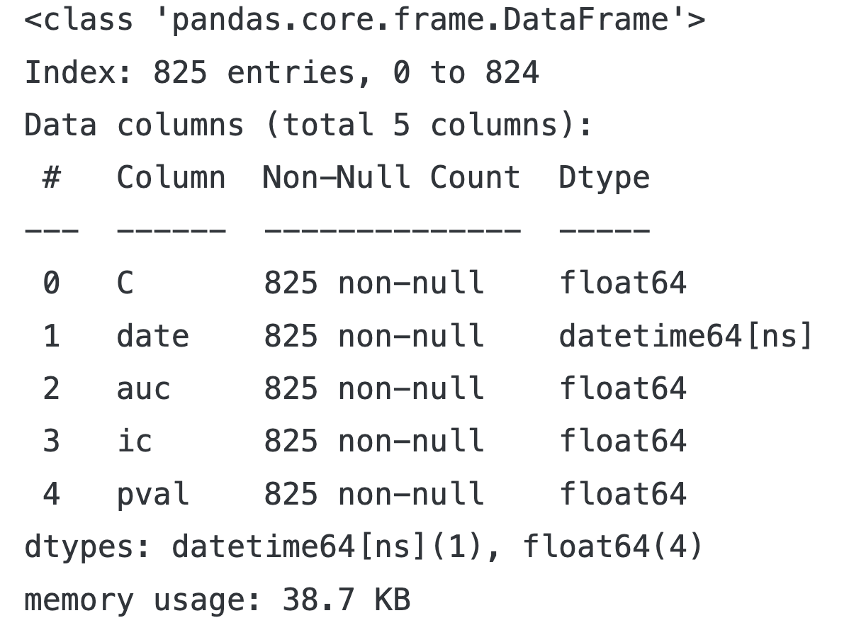

	count	mean	std	min	25%	50%	75%	max
C
0.00001	75.0	0.524834	0.033162	0.462730	0.500238	0.520174	0.543183	0.608531
0.00010	75.0	0.525391	0.033182	0.465664	0.500457	0.520052	0.539332	0.617832
0.00100	75.0	0.525726	0.034815	0.442510	0.499963	0.521454	0.546595	0.637523
0.01000	75.0	0.525146	0.036003	0.447376	0.500513	0.519809	0.547387	0.633047
0.10000	75.0	0.523507	0.036001	0.439579	0.501279	0.517053	0.548712	0.617858
1.00000	75.0	0.523068	0.035935	0.438185	0.500740	0.516178	0.548256	0.614613
10.00000	75.0	0.523020	0.035928	0.438122	0.500564	0.516100	0.548231	0.614639
100.00000	75.0	0.523012	0.035928	0.438088	0.500543	0.516050	0.548237	0.614629
1000.00000	75.0	0.523011	0.035929	0.438074	0.500541	0.516038	0.548239	0.614629
10000.00000	75.0	0.523010	0.035929	0.438079	0.500541	0.516038	0.548239	0.614629
100000.00000	75.0	0.523010	0.035929	0.438079	0.500541	0.516038	0.548239	0.614629

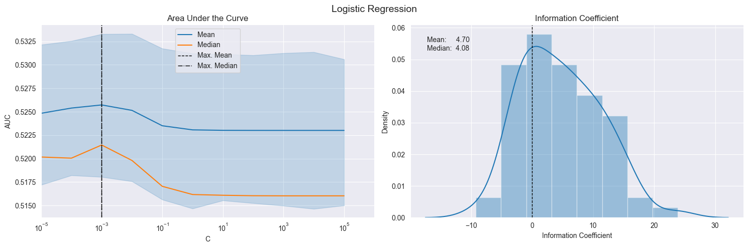
五、Plot Validation Scores 绘制验证分数

def plot_ic_distribution(df, ax=None):if ax is not None:sns.distplot(df.ic, ax=ax)    else:ax = sns.distplot(df.ic)mean, median = df.ic.mean(), df.ic.median()ax.axvline(0, lw=1, ls='--', c='k')ax.text(x=.05, y=.9, s=f'Mean: {mean:8.2f}\nMedian: {median:5.2f}',horizontalalignment='left',verticalalignment='center',transform=ax.transAxes)ax.set_xlabel('Information Coefficient')sns.despine()plt.tight_layout()fig, axes= plt.subplots(ncols=2, figsize=(15, 5))sns.lineplot(x='C', y='auc', data=log_scores, estimator=np.mean, label='Mean', ax=axes[0])
by_alpha = log_scores.groupby('C').auc.agg(['mean', 'median'])
best_auc = by_alpha['mean'].idxmax()
by_alpha['median'].plot(logx=True, ax=axes[0], label='Median', xlim=(10e-6, 10e5))
axes[0].axvline(best_auc, ls='--', c='k', lw=1, label='Max. Mean')
axes[0].axvline(by_alpha['median'].idxmax(), ls='-.', c='k', lw=1, label='Max. Median')
axes[0].legend()
axes[0].set_ylabel('AUC')
axes[0].set_xscale('log')
axes[0].set_title('Area Under the Curve')plot_ic_distribution(log_scores[log_scores.C==best_auc], ax=axes[1])
axes[1].set_title('Information Coefficient')fig.suptitle('Logistic Regression', fontsize=14)
sns.despine()
fig.tight_layout()
fig.subplots_adjust(top=.9);