ego(8)---L-BFGS优化算法与B样条生成最终轨迹

在经过上一步的为 Astar 路径点计算避障基准点与排斥方向后，就会在经过一道带避障约束的优化步骤，得到可以避障的轨迹控制点。

这部分的内容也是一个循环迭代的过程，循环调用 L-BFGS 优化器与 B 样条，检测是否满足避障条件。不满足则继续循环优化与B样条。

L-BFGS简述

关于优化算法，比较常用的就是梯度下降，高斯牛顿，LM。这部分可以看我之前记录的一篇博客：

https://blog.csdn.net/a_xiaoning/article/details/131276904

梯度下降的搜索方向为：

仅使用目标函数的一阶导数来确定搜索方向。

LM 算法做了改进，将搜索方向公式改为：

J 为雅可比矩阵。

区别

只需要抓住核心的区别即可，BFGS 又引入了一个海森矩阵 H ，使用一个公式来迭代计算 H 矩阵：

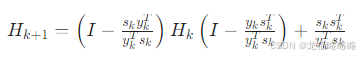
H 矩阵能够反应目标函数的曲率(二阶特性)，可以收敛更快。但缺点就是需要存储 n×n 的矩阵 H ，如果 n 很大的时候，也就是数据量特别大的时候，就需要特别大的内存。

因此 L-BFGS 就是放弃存储完整的 H 矩阵，指存储近期迭代的 si 与 yi ，来间接计算 H 矩阵。

关于 L-BFGS 的原理解释可以看这一篇博客：https://blog.csdn.net/weixin_39445556/article/details/84502260

写得挺好的，通俗易懂。

代价函数

比较关键的部分是代价函数的确立，在上一步的避障基准点数据与排斥方向也是用在代价函数中：

  // L-BFGS 求解器参数配置lbfgs::lbfgs_parameter_t lbfgs_params;lbfgs::lbfgs_load_default_parameters(&lbfgs_params);lbfgs_params.mem_size = 16; // 存储大小lbfgs_params.max_iterations = 200;  // 最大迭代次数lbfgs_params.g_epsilon = 0.01;  // 梯度收敛阈值(小于次值认为收敛)/* ---------- optimize ---------- */t1 = ros::Time::now();// 传入 costFunctionRebound 代价函数，此函数中会包含避障代价的计算int result = lbfgs::lbfgs_optimize(variable_num_, q, &final_cost, BsplineOptimizer::costFunctionRebound, NULL, BsplineOptimizer::earlyExit, this, &lbfgs_params);t2 = ros::Time::now();

代价函数就是其中的 BsplineOptimizer::costFunctionRebound 函数。

代价主要包括三个部分：

1. 平滑性代价

2. 避障代价

3. 可行性代价

void BsplineOptimizer::combineCostRebound(const double *x, double *grad, double &f_combine, const int n)
{memcpy(cps_.points.data() + 3 * order_, x, n * sizeof(x[0]));/* ---------- evaluate cost and gradient ---------- */double f_smoothness, f_distance, f_feasibility;Eigen::MatrixXd g_smoothness = Eigen::MatrixXd::Zero(3, cps_.size);Eigen::MatrixXd g_distance = Eigen::MatrixXd::Zero(3, cps_.size);Eigen::MatrixXd g_feasibility = Eigen::MatrixXd::Zero(3, cps_.size);calcSmoothnessCost(cps_.points, f_smoothness, g_smoothness);  // 平滑性代价calcDistanceCostRebound(cps_.points, f_distance, g_distance, iter_num_, f_smoothness);  // 避障代价calcFeasibilityCost(cps_.points, f_feasibility, g_feasibility); // 可行性代价f_combine = lambda1_ * f_smoothness + new_lambda2_ * f_distance + lambda3_ * f_feasibility;//printf("origin %f %f %f %f\n", f_smoothness, f_distance, f_feasibility, f_combine);Eigen::MatrixXd grad_3D = lambda1_ * g_smoothness + new_lambda2_ * g_distance + lambda3_ * g_feasibility;memcpy(grad, grad_3D.data() + 3 * order_, n * sizeof(grad[0]));
}

平滑性代价

这一点应用了B样条的高阶导数与离散差分类似，所以其核心思想是用相邻控制点的线性组合来近似连续轨迹的加加速度或加速度。

在 ego 中提供了两种代价计算，一种是加加1.速度，一种是加速度，默认是加加速度。

其推导也特别简单，就直接认为微分就是离散差值：

1.一阶导数(速度)

2.二阶导数(加速度)

3.三阶导数(加加速度)

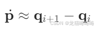
最后整理就可以得到：

代价就使用求得的加加速度去平方再加和。

在 ego 中除了这样计算代价外，还会同时利用代价来计算梯度，用于优化算法确定后续的收敛方向：

  // 平滑性代价  q--- B 样条控制点矩阵// 核心思想，离散差分近似导数，用两个相邻离散控制点的差值来近似连续曲线的导数void BsplineOptimizer::calcSmoothnessCost(const Eigen::MatrixXd &q, double &cost,Eigen::MatrixXd &gradient, bool falg_use_jerk /* = true*/){cost = 0.0;// 使用加加速度指标if (falg_use_jerk){Eigen::Vector3d jerk, temp_j;// 假设B样条曲线的时间/节点均匀，则第 i 个节点的加加速度可以通过 4 个连续控制点的 4 点差分近似// jerk = q.col(i + 3) - 3 * q.col(i + 2) + 3 * q.col(i + 1) - q.col(i);// 平滑性代价为所有加加速度的平方和 cost = sum(jerk^2)for (int i = 0; i < q.cols() - 3; i++){/* evaluate jerk */jerk = q.col(i + 3) - 3 * q.col(i + 2) + 3 * q.col(i + 1) - q.col(i);cost += jerk.squaredNorm();temp_j = 2.0 * jerk;/* jerk gradient */// 根据上述公式的系数来为代价来添加系数，存储在 gradient，作为优化器的梯度来计算后续的优化方向gradient.col(i + 0) += -temp_j;gradient.col(i + 1) += 3.0 * temp_j;gradient.col(i + 2) += -3.0 * temp_j;gradient.col(i + 3) += temp_j;}}// 使用加速度指标else{Eigen::Vector3d acc, temp_acc;for (int i = 0; i < q.cols() - 2; i++){/* evaluate acc */acc = q.col(i + 2) - 2 * q.col(i + 1) + q.col(i);cost += acc.squaredNorm();temp_acc = 2.0 * acc;/* acc gradient */gradient.col(i + 0) += temp_acc;gradient.col(i + 1) += -2.0 * temp_acc;gradient.col(i + 2) += temp_acc;}}}

避障代价

避障代价计算就比较简单了，因为已经有了避障基准点与排斥方向，就可以直接计算到障碍物的距离，然后根据距离的远近来确定不同的代价函数：

    /*** calculate distance cost and gradient ***/for (auto i = order_; i < end_idx; ++i)   // 避开边界点，与 B 样条阶数有关{// 遍历该控制点对应的所有障碍物for (size_t j = 0; j < cps_.direction[i].size(); ++j){double dist = (cps_.points.col(i) - cps_.base_point[i][j]).dot(cps_.direction[i][j]);   // 控制点到障碍物基准点的距离double dist_err = cps_.clearance - dist;  // 与安全距离阈值的误差  大于0则表示距离不足，需要提高代价来惩罚Eigen::Vector3d dist_grad = cps_.direction[i][j];if (dist_err < 0) // 避障距离足够时，不需要提升代价{/* do nothing */}else if (dist_err < demarcation)    // 距离不足但没有严重不足{cost += pow(dist_err, 3); // 代价使用误差的 3 次方gradient.col(i) += -3.0 * dist_err * dist_err * dist_grad;   // 避障的优化梯度，-3 * 误差 * 避障方向}else  // 距离严重不足{cost += a * dist_err * dist_err + b * dist_err + c; // 使用二次函数来计算代价，避免3次方后，代价过大gradient.col(i) += -(2.0 * a * dist_err + b) * dist_grad;}}}

可行性代价

可行性代价主要是判断动力学约束，判断轨迹是否满足无人机实际的速度与加速度约束，确保飞机能够实际跟上轨迹。

同样的，也是使用控制点差分，再除以B样条的时间间隔，就得到速度与加速度，再与最大速度，最大加速度进行判断，代码也比较容易理解：

    cost = 0.0;/* abbreviation */double ts, /*vm2, am2, */ ts_inv2;// vm2 = max_vel_ * max_vel_;// am2 = max_acc_ * max_acc_;ts = bspline_interval_;ts_inv2 = 1 / ts / ts;/* velocity feasibility */for (int i = 0; i < q.cols() - 1; i++){Eigen::Vector3d vi = (q.col(i + 1) - q.col(i)) / ts;  // 计算规划速度//cout << "temp_v * vi=" ;for (int j = 0; j < 3; j++){if (vi(j) > max_vel_){// cout << "fuck VEL" << endl;// cout << vi(j) << endl;cost += pow(vi(j) - max_vel_, 2) * ts_inv2; // multiply ts_inv3 to make vel and acc has similar magnitudegradient(j, i + 0) += -2 * (vi(j) - max_vel_) / ts * ts_inv2;gradient(j, i + 1) += 2 * (vi(j) - max_vel_) / ts * ts_inv2;}else if (vi(j) < -max_vel_){cost += pow(vi(j) + max_vel_, 2) * ts_inv2;gradient(j, i + 0) += -2 * (vi(j) + max_vel_) / ts * ts_inv2;gradient(j, i + 1) += 2 * (vi(j) + max_vel_) / ts * ts_inv2;}else{/* code */}}}/* acceleration feasibility */for (int i = 0; i < q.cols() - 2; i++){// 计算加速度Eigen::Vector3d ai = (q.col(i + 2) - 2 * q.col(i + 1) + q.col(i)) * ts_inv2;//cout << "temp_a * ai=" ;for (int j = 0; j < 3; j++){if (ai(j) > max_acc_){// cout << "fuck ACC" << endl;// cout << ai(j) << endl;cost += pow(ai(j) - max_acc_, 2);gradient(j, i + 0) += 2 * (ai(j) - max_acc_) * ts_inv2;gradient(j, i + 1) += -4 * (ai(j) - max_acc_) * ts_inv2;gradient(j, i + 2) += 2 * (ai(j) - max_acc_) * ts_inv2;}else if (ai(j) < -max_acc_){cost += pow(ai(j) + max_acc_, 2);gradient(j, i + 0) += 2 * (ai(j) + max_acc_) * ts_inv2;gradient(j, i + 1) += -4 * (ai(j) + max_acc_) * ts_inv2;gradient(j, i + 2) += 2 * (ai(j) + max_acc_) * ts_inv2;}else{/* code */}}//cout << endl;}