(LoRA深度解析)LORA: LOW-RANK ADAPTATION OF LARGE LANGUAGE MODELS论文精读(逐段解析)
LORA: LOW-RANK ADAPTATION OF LARGE LANGUAGE MODELS
LORA:大型语言模型的低秩适应
论文地址:https://arxiv.org/abs/2106.09685
官仓地址:https://github.com/microsoft/LoRA
微软公司
2021
【论文总结】
LoRA是一种参数高效的模型适配方法,基于权重变化具有低内在秩的假设,算法通过将权重更新矩阵ΔW\Delta WΔW分解为两个低秩矩阵A∈Rd×rA \in \mathbb{R}^{d \times r}A∈Rd×r和B∈Rr×kB \in \mathbb{R}^{r \times k}B∈Rr×k的乘积,其中r≪min(d,k)r \ll \min(d,k)r≪min(d,k),从而将原本需要d×kd \times kd×k个参数的更新压缩到(d+k)×r(d+k) \times r(d+k)×r个参数。在训练过程中,原始预训练权重W0W_0W0保持冻结,只训练低秩矩阵AAA和BBB,前向传播时输出为h=W0x+BAxh = W_0x + BAxh=W0x+BAx。这种设计使得LoRA能够实现高达10,000倍的参数压缩(如GPT-3 175B从350GB减少到35MB),同时保持与全参数微调相当的性能,且推理时可将BABABA与W0W_0W0合并,实现零延迟开销。算法特别适用于Transformer架构中的注意力权重矩阵,通过仅适配WqW_qWq和WvW_vWv矩阵即可获得最佳效果,验证了权重变化低秩假设的合理性。
ABSTRACT
An important paradigm of natural language processing consists of large-scale pretraining on general domain data and adaptation to particular tasks or domains. As we pre-train larger models, full fine-tuning, which retrains all model parameters, becomes less feasible. Using GPT-3 175B as an example – deploying independent instances of fine-tuned models, each with 175B parameters, is prohibitively expensive. We propose Low-Rank Adaptation, or LoRA, which freezes the pretrained model weights and injects trainable rank decomposition matrices into each layer of the Transformer architecture, greatly reducing the number of trainable parameters for downstream tasks. Compared to GPT-3 175B fine-tuned with Adam, LoRA can reduce the number of trainable parameters by 10,000 times and the GPU memory requirement by 3 times. LoRA performs on-par or better than finetuning in model quality on RoBERTa, DeBERTa, GPT-2, and GPT-3, despite having fewer trainable parameters, a higher training throughput, and, unlike adapters, no additional inference latency. We also provide an empirical investigation into rank-deficiency in language model adaptation, which sheds light on the efficacy of LoRA. We release a package that facilitates the integration of LoRA with PyTorch models and provide our implementations and model checkpoints for RoBERTa, DeBERTa, and GPT-2 at https://github.com/microsoft/LoRA.
【翻译】自然语言处理的一个重要范式包括在通用领域数据上进行大规模预训练,然后适配到特定任务或领域。随着我们预训练的模型越来越大,全参数微调(重新训练所有模型参数)变得越来越不可行。以GPT-3 175B为例——部署独立的微调模型实例,每个都有175B参数,成本高得令人望而却步。我们提出了低秩适配(Low-Rank Adaptation,LoRA),它冻结预训练模型权重,并在Transformer架构的每一层中注入可训练的秩分解矩阵,大大减少了下游任务的可训练参数数量。与使用Adam微调的GPT-3 175B相比,LoRA可以将可训练参数数量减少10,000倍,GPU内存需求减少3倍。LoRA在RoBERTa、DeBERTa、GPT-2和GPT-3上的模型质量表现与微调相当或更好,尽管可训练参数更少、训练吞吐量更高,并且与适配器不同,没有额外的推理延迟。我们还提供了关于语言模型适配中秩缺陷的实证研究,这揭示了LoRA有效性的原理。我们发布了一个便于将LoRA与PyTorch模型集成的包,并在 https://github.com/microsoft/LoRA 提供了我们在RoBERTa、DeBERTa和GPT-2上的实现和模型检查点。
【解析】现代自然语言处理遵循"预训练-微调"的两阶段范式,首先在大规模通用数据上进行预训练获得基础语言表示能力,然后针对具体任务进行微调。然而,随着模型规模急剧增长,传统的全参数微调面临严重挑战。全参数微调需要为每个下游任务维护一个完整的模型副本,当模型达到GPT-3的175B参数量级时,这种做法在存储和部署上都极其昂贵。LoRA的核心思想是基于这样一个假设:模型适配过程中的权重变化具有低内在维度特性。因此,LoRA不直接更新原始权重矩阵,而是学习一个低秩分解表示这些变化。具体来说,对于权重矩阵W∈Rd×kW \in \mathbb{R}^{d \times k}W∈Rd×k,LoRA将其更新ΔW\Delta WΔW分解为两个低秩矩阵A∈Rd×rA \in \mathbb{R}^{d \times r}A∈Rd×r和B∈Rr×kB \in \mathbb{R}^{r \times k}B∈Rr×k的乘积,其中r≪min(d,k)r \ll \min(d,k)r≪min(d,k)。这样,原本需要d×kd \times kd×k个参数的更新现在只需要(d+k)×r(d+k) \times r(d+k)×r个参数,实现了参数量的大幅压缩。更重要的是,LoRA保持了与全参数微调相当的性能表现,这验证了权重变化低秩假设的合理性。同时,LoRA的线性设计使得在推理时可以将学习到的低秩矩阵与原始权重合并,避免了额外的计算开销。
1 INTRODUCTION
Many applications in natural language processing rely on adapting one large-scale, pre-trained language model to multiple downstream applications. Such adaptation is usually done via fine-tuning, which updates all the parameters of the pre-trained model. The major downside of fine-tuning is that the new model contains as many parameters as in the original model. As larger models are trained every few months, this changes from a mere “inconvenience” for GPT-2 (Radford et al., b) or RoBERTa large (Liu et al., 2019) to a critical deployment challenge for GPT-3 (Brown et al., 2020) with 175 billion trainable parameters.
【翻译】自然语言处理中的许多应用都依赖于将一个大规模的预训练语言模型适配到多个下游应用中。这种适配通常通过微调来完成,微调会更新预训练模型的所有参数。微调的主要缺点是新模型包含与原始模型一样多的参数。随着每隔几个月就训练出更大的模型,这种情况从GPT-2或RoBERTa large的单纯"不便"变成了具有1750亿可训练参数的GPT-3的关键部署挑战。
Many sought to mitigate this by adapting only some parameters or learning external modules for new tasks. This way, we only need to store and load a small number of task-specific parameters in addition to the pre-trained model for each task, greatly boosting the operational efficiency when deployed. However, existing techniques often introduce inference latency (Houlsby et al., 2019; Rebuffi et al., 2017) by extending model depth or reduce the model’s usable sequence length (Li & Liang, 2021; Lester et al., 2021; Hambardzumyan et al., 2020; Liu et al., 2021) (Section 3). More importantly, these method often fail to match the fine-tuning baselines, posing a trade-off between efficiency and model quality.
【翻译】许多人试图通过仅适配部分参数或为新任务学习外部模块来缓解这个问题。这样,我们只需要为每个任务存储和加载少量特定任务的参数,除了预训练模型之外,大大提升了部署时的运营效率。然而,现有技术往往通过扩展模型深度引入推理延迟,或者减少模型的可用序列长度。更重要的是,这些方法往往无法达到微调基线的性能,在效率和模型质量之间构成了权衡。
【解析】面对全参数微调的扩展性问题,研究者们提出了各种参数高效的适配方法。这些方法的核心思想是固定预训练模型的主体参数,只学习和存储少量特定任务的参数。这种策略的优势显而易见:可以显著降低存储需求和部署成本,因为多个任务可以共享同一个预训练模型主体,只需要为每个任务维护很小的特定参数集。然而,这些早期的参数高效方法面临两个主要挑战。首先是推理效率问题,许多方法通过在原有架构中插入适配器层或修改输入表示来实现参数高效,但这些修改往往增加了模型的计算路径长度或改变了原有的并行计算模式,导致推理时间增加。其次是性能降级问题,这些方法通常在效率提升的同时伴随着任务性能的下降,无法完全匹配全参数微调的效果。
Figure 1: Our reparametrization. We only train AAA and BBB .
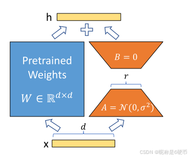
【翻译】图1:我们的重参数化方法。我们只训练矩阵AAA和BBB。
【解析】这个图示展示了LoRA方法。在传统的全参数微调中,我们需要直接更新权重矩阵WWW。而LoRA提出了一种巧妙的重参数化策略:保持原始权重矩阵WWW冻结不变,转而学习两个低秩矩阵AAA和BBB。在前向传播过程中,输入xxx同时通过原始路径WxWxWx和新增的低秩路径B(Ax)B(Ax)B(Ax),最终输出为两者之和。这种设计的关键在于矩阵AAA和BBB的秩rrr远小于原始权重矩阵的维度,因此参数量大幅减少。同时,由于这种线性组合的设计,在部署时可以将BABABA与WWW直接相加得到新的权重矩阵,从而避免了推理时的额外计算开销。
我这里补充一下相关知识
【矩阵的秩(Rank)基础知识以及LoRA使用】
为了深入理解LoRA的核心原理,我们需要从矩阵的秩这一基础概念开始。矩阵的秩是线性代数中的一个重要概念,它描述了矩阵所包含的线性无关信息的"维度"或"复杂度"。
1. 矩阵秩的定义
矩阵的秩等于其行向量(或列向量)中线性无关向量的最大个数。对于一个m×nm \times nm×n的矩阵MMM,其秩rank(M)≤min(m,n)\text{rank}(M) \leq \min(m,n)rank(M)≤min(m,n)。
2. 直观理解的话
可以将矩阵的秩理解为矩阵所能表达的"独立信息"的数量。例如:
- 满秩矩阵:包含最大可能的独立信息
- 低秩矩阵:包含的独立信息较少,存在冗余
具体计算实例:
让我们通过具体例子来理解矩阵秩的计算:
实例1:计算矩阵的秩
A=(123246112)A = \begin{pmatrix} 1 & 2 & 3 \\ 2 & 4 & 6 \\ 1 & 1 & 2 \end{pmatrix}A=121241362
让我们详细计算高斯消元的过程:
步骤1:写出原始矩阵
A=(123246112)A = \begin{pmatrix} 1 & 2 & 3 \\ 2 & 4 & 6 \\ 1 & 1 & 2 \end{pmatrix}A=121241362
步骤2:第一轮消元(消除第一列下方的元素)
- 对第二行进行操作:R2←R2−2R1R_2 \leftarrow R_2 - 2R_1R2←R2−2R1
- 对第三行进行操作:R3←R3−R1R_3 \leftarrow R_3 - R_1R3←R3−R1
具体计算:
- 新的第二行:(2,4,6)−2(1,2,3)=(2−2,4−4,6−6)=(0,0,0)(2,4,6) - 2(1,2,3) = (2-2, 4-4, 6-6) = (0,0,0)(2,4,6)−2(1,2,3)=(2−2,4−4,6−6)=(0,0,0)
- 新的第三行:(1,1,2)−(1,2,3)=(1−1,1−2,2−3)=(0,−1,−1)(1,1,2) - (1,2,3) = (1-1, 1-2, 2-3) = (0,-1,-1)(1,1,2)−(1,2,3)=(1−1,1−2,2−3)=(0,−1,−1)
得到:
(1230000−1−1)\begin{pmatrix} 1 & 2 & 3 \\ 0 & 0 & 0 \\ 0 & -1 & -1 \end{pmatrix}10020−130−1
步骤3:交换行(将零行移到最后)
交换第二行和第三行:R2↔R3R_2 \leftrightarrow R_3R2↔R3
(1230−1−1000)\begin{pmatrix} 1 & 2 & 3 \\ 0 & -1 & -1 \\ 0 & 0 & 0 \end{pmatrix}1002−103−10
步骤4:规范化第二行
将第二行乘以-1:R2←−R2R_2 \leftarrow -R_2R2←−R2
(123011000)\begin{pmatrix} 1 & 2 & 3 \\ 0 & 1 & 1 \\ 0 & 0 & 0 \end{pmatrix}100210310
步骤5:第二轮消元(消除第二列上方的元素)
对第一行进行操作:R1←R1−2R2R_1 \leftarrow R_1 - 2R_2R1←R1−2R2
具体计算:(1,2,3)−2(0,1,1)=(1,2−2,3−2)=(1,0,1)(1,2,3) - 2(0,1,1) = (1,2-2,3-2) = (1,0,1)(1,2,3)−2(0,1,1)=(1,2−2,3−2)=(1,0,1)
最终得到简化行阶梯形式(rref):
rref(A)=(101011000)\text{rref}(A) = \begin{pmatrix} 1 & 0 & 1 \\ 0 & 1 & 1 \\ 0 & 0 & 0 \end{pmatrix}rref(A)=100010110
步骤6:确定矩阵的秩
从简化行阶梯形式可以看出:
rref(A)=(101011000)\text{rref}(A) = \begin{pmatrix} 1 & 0 & 1 \\ 0 & 1 & 1 \\ 0 & 0 & 0 \end{pmatrix}rref(A)=100010110
矩阵的秩等于其简化行阶梯形式中非零行的数量:
- 第一行:(1,0,1)≠(0,0,0)(1,0,1) \neq (0,0,0)(1,0,1)=(0,0,0),非零行
- 第二行:(0,1,1)≠(0,0,0)(0,1,1) \neq (0,0,0)(0,1,1)=(0,0,0),非零行
- 第三行:(0,0,0)(0,0,0)(0,0,0),零行
所以rank(A)=2\text{rank}(A) = 2rank(A)=2(有2个非零行),这是一个低秩矩阵。
实例2:LoRA中的参数量对比
假设我们有一个Transformer中的注意力权重矩阵Wq∈R768×768W_q \in \mathbb{R}^{768 \times 768}Wq∈R768×768:
原始全参数微调方式:
- 需要更新整个权重矩阵WqW_qWq
- 可训练参数量:768×768=589,824768 \times 768 = 589,824768×768=589,824个参数
LoRA方式:
冻结原始权重WqW_qWq,只训练低秩分解矩阵,设秩r=8r = 8r=8:
- 矩阵A∈Rr×dinA \in \mathbb{R}^{r \times d_{in}}A∈Rr×din,即A∈R8×768A \in \mathbb{R}^{8 \times 768}A∈R8×768:8×768=6,1448 \times 768 = 6,1448×768=6,144个参数
- 矩阵B∈Rdout×rB \in \mathbb{R}^{d_{out} \times r}B∈Rdout×r,即B∈R768×8B \in \mathbb{R}^{768 \times 8}B∈R768×8:768×8=6,144768 \times 8 = 6,144768×8=6,144个参数
- LoRA总参数量:6,144+6,144=12,2886,144 + 6,144 = 12,2886,144+6,144=12,288个参数
计算原理:
更新后的权重为:Wq′=Wq+ΔW=Wq+BAW_q' = W_q + \Delta W = W_q + BAWq′=Wq+ΔW=Wq+BA
其中ΔW=BA\Delta W = BAΔW=BA是低秩更新,维度验证:
BA:R768×8×R8×768=R768×768BA: \mathbb{R}^{768 \times 8} \times \mathbb{R}^{8 \times 768} = \mathbb{R}^{768 \times 768}BA:R768×8×R8×768=R768×768
参数效率对比:
- 参数压缩比:589,82412,288≈48\frac{589,824}{12,288} \approx 4812,288589,824≈48倍
- 参数减少率:589,824−12,288589,824×100%≈97.9%\frac{589,824 - 12,288}{589,824} \times 100\% \approx 97.9\%589,824589,824−12,288×100%≈97.9%
- 仅需训练原参数量的12,288589,824×100%≈2.1%\frac{12,288}{589,824} \times 100\% \approx 2.1\%589,82412,288×100%≈2.1%
实例3:不同秩值的影响
对于同样的768×768768 \times 768768×768矩阵,不同的秩值rrr对应的参数量:
计算公式:
- 原始矩阵参数量:768×768=589,824768 \times 768 = 589,824768×768=589,824个参数
- LoRA参数量:矩阵A∈Rr×768A \in \mathbb{R}^{r \times 768}A∈Rr×768和矩阵B∈R768×rB \in \mathbb{R}^{768 \times r}B∈R768×r的总参数量为r×768+768×r=2×768×rr \times 768 + 768 \times r = 2 \times 768 \times rr×768+768×r=2×768×r
- 压缩比 = 原始参数量LoRA参数量=589,8242×768×r=589,8241,536×r\frac{\text{原始参数量}}{\text{LoRA参数量}} = \frac{589,824}{2 \times 768 \times r} = \frac{589,824}{1,536 \times r}LoRA参数量原始参数量=2×768×r589,824=1,536×r589,824
具体计算如下:
- r=1r = 1r=1:
- LoRA参数量:2×768×1=1,5362 \times 768 \times 1 = 1,5362×768×1=1,536个参数
- 压缩比:589,8241,536=384\frac{589,824}{1,536} = 3841,536589,824=384倍
- r=4r = 4r=4:
- LoRA参数量:2×768×4=6,1442 \times 768 \times 4 = 6,1442×768×4=6,144个参数
- 压缩比:589,8246,144=96\frac{589,824}{6,144} = 966,144589,824=96倍
- r=16r = 16r=16:
- LoRA参数量:2×768×16=24,5762 \times 768 \times 16 = 24,5762×768×16=24,576个参数
- 压缩比:589,82424,576=24\frac{589,824}{24,576} = 2424,576589,824=24倍
- r=64r = 64r=64:
- LoRA参数量:2×768×64=98,3042 \times 768 \times 64 = 98,3042×768×64=98,304个参数
- 压缩比:589,82498,304=6\frac{589,824}{98,304} = 698,304589,824=6倍
可以看出
- 随着秩rrr的增加,参数量线性增长:参数量=1,536×r\text{参数量} = 1,536 \times r参数量=1,536×r
- 压缩比反比例下降:压缩比=384r\text{压缩比} = \frac{384}{r}压缩比=r384
- 更高的秩提供更强的表达能力,但牺牲了参数效率
实例4:在轻量化模型中的应用
假如我们要使用的是Qwen2-1.5B模型:
- 假设隐藏维度dmodel=1536d_{model} = 1536dmodel=1536
- 注意力投影矩阵Wq,Wk,Wv,Wo∈R1536×1536W_q, W_k, W_v, W_o \in \mathbb{R}^{1536 \times 1536}Wq,Wk,Wv,Wo∈R1536×1536
- 每个矩阵原始参数量:15362=2,359,2961536^2 = 2,359,29615362=2,359,296
- 使用r=8r = 8r=8的LoRA:2×1536×8=24,5762 \times 1536 \times 8 = 24,5762×1536×8=24,576个参数
- 压缩比:2,359,29624,576≈96\frac{2,359,296}{24,576} \approx 9624,5762,359,296≈96倍
其实到这里我们就可以了解为什么LoRA能够在保持性能的同时大幅减少可训练参数量。
3. 低秩分解的概念
任何矩阵M∈Rm×nM \in \mathbb{R}^{m \times n}M∈Rm×n如果其秩为rrr,都可以分解为两个矩阵的乘积:M=UVTM = UV^TM=UVT,其中U∈Rm×rU \in \mathbb{R}^{m \times r}U∈Rm×r,V∈Rn×rV \in \mathbb{R}^{n \times r}V∈Rn×r。
4. 参数量对比
这里是关键的效率提升来源:
- 原始矩阵参数量:m×nm \times nm×n
- 低秩分解参数量:m×r+n×r=(m+n)×rm \times r + n \times r = (m+n) \times rm×r+n×r=(m+n)×r
- 当r≪min(m,n)r \ll \min(m,n)r≪min(m,n)时,参数量大幅减少
5. LoRA中的应用
在LoRA中,假设权重更新ΔW\Delta WΔW具有低秩特性,因此用ΔW=BA\Delta W = BAΔW=BA来近似,其中A∈Rr×kA \in \mathbb{R}^{r \times k}A∈Rr×k,B∈Rd×rB \in \mathbb{R}^{d \times r}B∈Rd×r,r≪min(d,k)r \ll \min(d,k)r≪min(d,k)。这样就将原本需要d×kd \times kd×k个参数的更新压缩到(d+k)×r(d+k) \times r(d+k)×r个参数。
6. 为什么低秩假设合理呢?
研究发现,神经网络在适配新任务时,权重的变化往往集中在少数几个主要方向上,大部分方向上的变化很小或为零。这意味着权重更新矩阵ΔW\Delta WΔW确实具有低秩特性,LoRA正是利用了这一观察。
===继续回到原论文=
We take inspiration from Li et al. (2018a); Aghajanyan et al. (2020) which show that the learned over-parametrized models in fact reside on a low intrinsic dimension. We hypothesize that the change in weights during model adaptation also has a low “intrinsic rank”, leading to our proposed Low-Rank Adaptation (LoRA) approach. LoRA allows us to train some dense layers in a neural network indirectly by optimizing rank decomposition matrices of the dense layers’ change during adaptation instead, while keeping the pre-trained weights frozen, as shown in Figure 1. Using GPT-3 175B as an example, we show that a very low rank (i.e., rrr in Figure 1 can be one or two) suffices even when the full rank (i.e., ddd ) is as high as 12,288, making LoRA both storage- and compute-efficient.
【翻译】我们从Li et al. (2018a)和Aghajanyan et al. (2020)的研究中获得启发,他们表明学习到的过参数化模型实际上存在于一个低内在维度中。我们假设模型适配期间权重的变化也具有低"内在秩",从而提出了我们的低秩适配(LoRA)方法。LoRA允许我们通过优化密集层在适配过程中变化的秩分解矩阵来间接训练神经网络中的一些密集层,同时保持预训练权重冻结,如图1所示。以GPT-3 175B为例,我们展示了即使当满秩(即ddd)高达12,288时,非常低的秩(即图1中的rrr可以是一或二)就足够了,这使得LoRA在存储和计算上都是高效的。
【解析】尽管现代神经网络包含数百万甚至数十亿个参数,但这些模型的有效信息实际上可以压缩到一个相对较低的维度空间中。这种现象被称为"低内在维度"特性,说明了模型的表示能力主要集中在少数几个关键方向上。基于这一观察,作者提出了一个关键假设:在模型适配过程中,权重的更新变化同样遵循低秩特性。这个假设具有重要的实际价值,因为如果权重变化ΔW\Delta WΔW确实是低秩的,那么我们就可以用两个小矩阵的乘积BABABA来近似表示这种变化,从而大幅减少需要训练的参数数量。LoRA的设计策略其实就是一种巧妙的间接优化思路:与其直接修改原始权重矩阵,不如学习描述权重变化的低秩分解。这种方法的有效性在GPT-3这样的超大规模模型上得到了验证,即使模型的隐藏维度达到12,288,仅使用秩为1或2的分解就能获得良好的适配效果,这充分证明了权重变化低秩假设的合理性。
LoRA possesses several key advantages.
• LoRA makes training more efficient and lowers the hardware barrier to entry by up to 3 times when using adaptive optimizers since we do not need to calculate the gradients or maintain the optimizer states for most parameters. Instead, we only optimize the injected, much smaller low-rank matrices.
• A pre-trained model can be shared and used to build many small LoRA modules for different tasks. We can freeze the shared model and efficiently switch tasks by replacing the matrices AAA and BBB in Figure 1, reducing the storage requirement and task-switching overhead significantly.
• Our simple linear design allows us to merge the trainable matrices with the frozen weights when deployed, introducing no inference latency compared to a fully fine-tuned model, by construction.
• LoRA is orthogonal to many prior methods and can be combined with many of them, such as prefix-tuning. We provide an example in Appendix E.
【翻译】LoRA具有几个关键优势。
【翻译】• 预训练模型可以被共享并用于构建许多针对不同任务的小型LoRA模块。我们可以冻结共享模型,并通过替换图1中的矩阵AAA和BBB来高效地切换任务,从而显著降低存储需求和任务切换开销。
【翻译】• LoRA使训练更加高效,并在使用自适应优化器时将硬件准入门槛降低了多达3倍,因为我们不需要为大部分参数计算梯度或维护优化器状态。相反,我们只优化注入的、更小的低秩矩阵。
【翻译】• 我们简单的线性设计允许我们在部署时将可训练矩阵与冻结权重合并,根据构造,与完全微调的模型相比不会引入推理延迟。
【翻译】• LoRA与许多先前的方法是正交的,可以与其中许多方法结合使用,例如前缀调优。我们在附录E中提供了一个例子。
【解析】"正交"在这里指的是LoRA与其他方法在技术实现上不存在冲突,可以同时应用而不会相互干扰。
Terminologies and Conventions. We make frequent references to the Transformer architecture and use the conventional terminologies for its dimensions. We call the input and output dimension size of a Transformer layer dmodeld_{m o d e l}dmodel . We use WqW_{q}Wq , WkW_{k}Wk , WvW_{v}Wv , and WoW_{o}Wo to refer to the query/key/value/output projection matrices in the self-attention module. WWW or W0W_{0}W0 refers to a pretrained weight matrix and ΔW\Delta WΔW its accumulated gradient update during adaptation. We use rrr to denote the rank of a LoRA module. We follow the conventions set out by (Vaswani et al., 2017; Brown et al., 2020) and use Adam (Loshchilov & Hutter, 2019; Kingma & Ba, 2017) for model optimization and use a Transformer MLP feedforward dimension dffn=4×dmodel{d_{f f n}}=4\times{d_{m o d e l}}dffn=4×dmodel .
【翻译】术语和约定。我们经常引用Transformer架构并使用其维度的常规术语。我们将Transformer层的输入和输出维度大小称为dmodeld_{model}dmodel。我们使用WqW_{q}Wq、WkW_{k}Wk、WvW_{v}Wv和WoW_{o}Wo来指代自注意力模块中的查询/键/值/输出投影矩阵。WWW或W0W_{0}W0指预训练权重矩阵,ΔW\Delta WΔW指其在适配期间的累积梯度更新。我们使用rrr来表示LoRA模块的秩。我们遵循(Vaswani et al., 2017; Brown et al., 2020)设定的约定,使用Adam (Loshchilov & Hutter, 2019; Kingma & Ba, 2017)进行模型优化,并使用Transformer MLP前馈维度dffn=4×dmodel{d_{ffn}}=4\times{d_{model}}dffn=4×dmodel。
【解析】在Transformer架构中,dmodeld_{model}dmodel是一个核心参数,它决定了模型的隐藏状态维度,直接影响模型的表达能力和计算复杂度。自注意力机制中的四个投影矩阵Wq,Wk,Wv,WoW_q, W_k, W_v, W_oWq,Wk,Wv,Wo是LoRA主要应用的目标,因为这些矩阵通常具有较大的参数量且对模型性能影响显著。符号ΔW\Delta WΔW表示权重的变化量,这正是LoRA方法要用低秩分解来近似的核心对象。参数rrr控制着LoRA的压缩程度和表达能力之间的平衡。MLP层的维度关系dffn=4×dmodel{d_{ffn}}=4\times{d_{model}}dffn=4×dmodel是Transformer的标准设计,4倍扩展为模型提供了充分的非线性变换能力。
2 问题陈述
While our proposal is agnostic to training objective, we focus on language modeling as our motivating use case. Below is a brief description of the language modeling problem and, in particular, the maximization of conditional probabilities given a task-specific prompt.
【翻译】虽然我们的提议对训练目标是不可知的,但我们专注于语言建模作为我们的激励用例。下面是语言建模问题的简要描述,特别是在给定任务特定提示的情况下条件概率的最大化。
【解析】这里的"不可知"是说LoRA方法具有通用性,不依赖于特定的训练目标函数,可以应用于各种不同的机器学习任务。作者选择语言建模作为主要研究对象,是因为它是当前大模型最重要的应用场景之一。语言建模的核心是预测下一个词的概率分布,而条件概率最大化是这一过程的数学表达。概率建模方式使得模型能够根据上下文信息生成连贯的文本序列。
Suppose we are given a pre-trained autoregressive language model PΦ(y∣x)P_{\Phi}(y|x)PΦ(y∣x) parametrized by Φ\PhiΦ . For instance, PΦ(y∣x)P_{\Phi}(y|x)PΦ(y∣x) can be a generic multi-task learner such as GPT (Radford et al., b; Brown et al., 2020) based on the Transformer architecture (Vaswani et al., 2017). Consider adapting this pre-trained model to downstream conditional text generation tasks, such as summarization, machine reading comprehension (MRC), and natural language to SQL (NL2SQL). Each downstream task is represented by a training dataset of context-target pairs: Z={(xi,yi)}i=1,..,N\mathcal{Z}=\{(x_{i},y_{i})\}_{i=1,..,N}Z={(xi,yi)}i=1,..,N , where both xix_{i}xi and yiy_{i}yi are sequences of tokens. For example, in NL2SQL, xix_{i}xi is a natural language query and yiy_{i}yi its corresponding SQL command; for summarization, xix_{i}xi is the content of an article and yiy_{i}yi its summary.
【翻译】假设我们有一个预训练的自回归语言模型PΦ(y∣x)P_{\Phi}(y|x)PΦ(y∣x),由参数Φ\PhiΦ参数化。例如,PΦ(y∣x)P_{\Phi}(y|x)PΦ(y∣x)可以是一个通用的多任务学习器,如基于Transformer架构(Vaswani et al., 2017)的GPT (Radford et al., b; Brown et al., 2020)。考虑将这个预训练模型适配到下游条件文本生成任务,如摘要、机器阅读理解(MRC)和自然语言转SQL(NL2SQL)。每个下游任务由上下文-目标对的训练数据集表示:Z={(xi,yi)}i=1,..,N\mathcal{Z}=\{(x_{i},y_{i})\}_{i=1,..,N}Z={(xi,yi)}i=1,..,N,其中xix_{i}xi和yiy_{i}yi都是token序列。例如,在NL2SQL中,xix_{i}xi是自然语言查询,yiy_{i}yi是其对应的SQL命令;对于摘要任务,xix_{i}xi是文章内容,yiy_{i}yi是其摘要。
【解析】自回归语言模型是按顺序生成文本,每次预测下一个token时都会考虑之前所有已生成的token。符号PΦ(y∣x)P_{\Phi}(y|x)PΦ(y∣x)表示在给定输入xxx的条件下生成输出yyy的概率分布,即条件概率建模。
During full fine-tuning, the model is initialized to pre-trained weights Φ0\Phi_{0}Φ0 and updated to Φ0+ΔΦ\Phi_{0}+\Delta\PhiΦ0+ΔΦ by repeatedly following the gradient to maximize the conditional language modeling objective:
【翻译】在全参数微调过程中,模型被初始化为预训练权重Φ0\Phi_{0}Φ0,并通过重复跟随梯度更新到Φ0+ΔΦ\Phi_{0}+\Delta\PhiΦ0+ΔΦ,以最大化条件语言建模目标:
【解析】Φ0\Phi_{0}Φ0代表从大规模预训练中获得的初始权重,ΔΦ\Delta\PhiΔΦ表示在特定任务上的参数更新量,它的维度与原始参数相同。梯度下降优化过程通过计算损失函数相对于参数的偏导数,确定参数更新的方向和幅度。这种"重复跟随梯度"的过程实际上是通过多轮迭代训练,让模型逐步适应新任务的数据分布和目标函数。
maxΦ∑(x,y)∈Z∑t=1∣y∣log(PΦ(yt∣x,y<t))\operatorname*{max}_{\Phi}\sum_{(x,y)\in\mathcal{Z}}\sum_{t=1}^{|y|}\log\left(P_{\Phi}(y_{t}|x,y_{<t})\right) Φmax(x,y)∈Z∑t=1∑∣y∣log(PΦ(yt∣x,y<t))
【解析】这个目标函数是最大似然估计的对数形式,将复杂的序列生成问题分解为逐个token的预测任务。外层求和遍历训练集中的所有样本对,内层求和针对目标序列中的每个位置进行建模。符号y<ty_{<t}y<t表示第ttt个位置之前的所有token。使用对数概率是为了便于数值计算,同时将概率的乘积转化为加法,避免数值下溢问题。最大化这个目标函数的过程就是让模型学会在给定上下文的条件下,为正确的下一个token分配更高的概率,从而实现准确的序列生成能力。
One of the main drawbacks for full fine-tuning is that for each downstream task, we learn a different set of parameters ΔΦ\Delta\PhiΔΦ whose dimension ∣ΔΦ∣|\Delta\Phi|∣ΔΦ∣ equals ∣Φ0∣\left|\Phi_{0}\right|∣Φ0∣ . Thus, if the pre-trained model is large (such as GPT-3 with ∣Φ0∣≈175|\Phi_{0}|\approx175∣Φ0∣≈175 Billion), storing and deploying many independent instances of fine-tuned models can be challenging, if at all feasible.
【翻译】全参数微调的主要缺点之一是,对于每个下游任务,我们学习一组不同的参数ΔΦ\Delta\PhiΔΦ,其维度∣ΔΦ∣|\Delta\Phi|∣ΔΦ∣等于∣Φ0∣\left|\Phi_{0}\right|∣Φ0∣。因此,如果预训练模型很大(例如具有∣Φ0∣≈175|\Phi_{0}|\approx175∣Φ0∣≈175亿参数的GPT-3),存储和部署许多独立的微调模型实例可能具有挑战性,甚至根本不可行。
In this paper, we adopt a more parameter-efficient approach, where the task-specific parameter increment ΔΦ=ΔΦ(Θ)\Delta\Phi=\Delta\Phi(\Theta)ΔΦ=ΔΦ(Θ) is further encoded by a much smaller-sized set of parameters Θ\ThetaΘ with ∣Θ∣≪∣Φ0∣|\Theta|\ll|\Phi_{0}|∣Θ∣≪∣Φ0∣ . The task of finding ΔΦ\Delta\PhiΔΦ thus becomes optimizing over Θ\ThetaΘ :
【翻译】在本文中,我们采用了一种更加参数高效的方法,其中任务特定的参数增量ΔΦ=ΔΦ(Θ)\Delta\Phi=\Delta\Phi(\Theta)ΔΦ=ΔΦ(Θ)被进一步编码为一个更小规模的参数集Θ\ThetaΘ,满足∣Θ∣≪∣Φ0∣|\Theta|\ll|\Phi_{0}|∣Θ∣≪∣Φ0∣。因此,寻找ΔΦ\Delta\PhiΔΦ的任务变成了对Θ\ThetaΘ的优化:
【解析】关键在于建立一个函数映射关系ΔΦ(Θ)\Delta\Phi(\Theta)ΔΦ(Θ),使得大维度的参数变化可以通过小维度的参数集来表示。符号∣Θ∣≪∣Φ0∣|\Theta|\ll|\Phi_{0}|∣Θ∣≪∣Φ0∣中的双小于号表示Θ\ThetaΘ的维度远小于原始参数。这种编码策略是假设参数变化具有低维结构,即高维空间中的变化实际上可以在低维子空间中有效表示。通过这种间接优化策略,我们不再直接更新所有原始参数,而是优化这个紧凑的参数表示Θ\ThetaΘ,然后通过映射函数生成所需的参数变化。这样就大幅减少了需要存储和优化的参数数量,同时保持了模型的表达能力。
maxΘ∑(x,y)∈Z∑t=1∣y∣log(pΦ0+ΔΦ(Θ)(yt∣x,y<t))\operatorname*{max}_{\Theta}\sum_{(x,y)\in\mathcal{Z}}\sum_{t=1}^{|y|}\log\left(p_{\Phi_{0}+\Delta\Phi(\Theta)}\bigl(y_{t}\bigl|x,y_{<t}\bigr)\right) Θmax(x,y)∈Z∑t=1∑∣y∣log(pΦ0+ΔΦ(Θ)(ytx,y<t))
【解析】优化目标函数。与传统微调不同,这里的优化变量从原始参数Φ\PhiΦ变为紧凑参数集Θ\ThetaΘ。模型的实际参数为Φ0+ΔΦ(Θ)\Phi_{0}+\Delta\Phi(\Theta)Φ0+ΔΦ(Θ),其中Φ0\Phi_0Φ0保持冻结,所有的适应性学习都通过Θ\ThetaΘ来实现。优化过程在低维空间中进行,显著降低了计算复杂度和内存需求。梯度计算只需要对Θ\ThetaΘ进行,而不需要对整个Φ\PhiΦ计算梯度,实现训练效率提升。
In the subsequent sections, we propose to use a low-rank representation to encode ΔΦ\Delta\PhiΔΦ that is both compute- and memory-efficient. When the pre-trained model is GPT-3 175B, the number of trainable parameters ∣Θ∣|\Theta|∣Θ∣ can be as small as 0.01%0.01\%0.01% of ∣Φ0∣\left|\Phi_{0}\right|∣Φ0∣ .
【翻译】在后续章节中,我们提出使用低秩表示来编码ΔΦ\Delta\PhiΔΦ,这种方法既计算高效又内存高效。当预训练模型是GPT-3 175B时,可训练参数的数量∣Θ∣|\Theta|∣Θ∣可以小到∣Φ0∣\left|\Phi_{0}\right|∣Φ0∣的0.01%0.01\%0.01%。
3 现有解决方案不够好吗?
The problem we set out to tackle is by no means new. Since the inception of transfer learning, dozens of works have sought to make model adaptation more parameter- and compute-efficient. See Section 6 for a survey of some of the well-known works. Using language modeling as an example, there are two prominent strategies when it comes to efficient adaptations: adding adapter layers (Houlsby et al., 2019; Rebuffi et al., 2017; Pfeiffer et al., 2021; Ricklé et al., 2020) or optimizing some forms of the input layer activations (Li & Liang, 2021; Lester et al., 2021; Hambardzumyan et al., 2020; Liu et al., 2021). However, both strategies have their limitations, especially in a large-scale and latency-sensitive production scenario.
【翻译】我们着手解决的问题绝不是新问题。自迁移学习出现以来,已有数十项工作致力于使模型适配更加参数高效和计算高效。参见第6节对一些知名工作的综述。以语言建模为例,在高效适配方面有两种突出的策略:添加适配器层(Houlsby et al., 2019; Rebuffi et al., 2017; Pfeiffer et al., 2021; Ricklé et al., 2020)或优化某些形式的输入层激活(Li & Liang, 2021; Lester et al., 2021; Hambardzumyan et al., 2020; Liu et al., 2021)。然而,这两种策略都有其局限性,特别是在大规模且对延迟敏感的生产场景中。
【解析】高效模型适配。
第一类方法是适配器架构,核心思想是在预训练模型的层间插入小型神经网络模块,这些适配器模块包含少量参数,专门负责学习特定任务的知识。预训练参数保持冻结,只训练适配器参数,从而实现参数高效的适配。
第二类方法是输入激活优化,包括前缀调优和提示调优等技术,这类方法不修改模型结构,而是通过优化输入表示来实现任务适配。前缀调优在输入序列前添加可学习的虚拟token,提示调优则直接优化连续的提示向量。虽然这些方法在学术研究中表现良好,但在实际生产环境中却难进行。大规模部署要求低推理延迟,而适配器层的顺序处理特性和输入优化方法的序列长度占用都会影响系统性能。
Adapter Layers Introduce Inference Latency. There are many variants of adapters. We focus on the original design by Houlsby et al. (2019) which has two adapter layers per Transformer block and a more recent one by Lin et al. (2020) which has only one per block but with an additional LayerNorm (Ba et al., 2016). While one can reduce the overall latency by pruning layers or exploiting multi-task settings (Ruicklé et al., 2020; Pfeiffer et al., 2021), there is no direct ways to bypass the extra compute in adapter layers. This seems like a non-issue since adapter layers are designed to have few parameters (sometimes <1%<1\%<1% of the original model) by having a small bottleneck dimension, which limits the FLOPs they can add. However, large neural networks rely on hardware parallelism to keep the latency low, and adapter layers have to be processed sequentially. This makes a difference in the online inference setting where the batch size is typically as small as one. In a generic scenario without model parallelism, such as running inference on GPT-2 (Radford et al., b) medium on a single GPU, we see a noticeable increase in latency when using adapters, even with a very small bottleneck dimension (Table 1).
【翻译】适配器层引入推理延迟。有许多适配器的变体。我们专注于Houlsby等人(2019)的原始设计,该设计在每个Transformer块中有两个适配器层,以及Lin等人(2020)的最新设计,该设计每个块只有一个适配器层但有额外的LayerNorm(Ba等人,2016)。虽然可以通过剪枝层或利用多任务设置来减少整体延迟(Ruicklé等人,2020;Pfeiffer等人,2021),但没有直接的方法绕过适配器层中的额外计算。这似乎不是问题,因为适配器层被设计为具有很少的参数(有时<1%<1\%<1%的原始模型),通过具有小的瓶颈维度来限制它们可以添加的FLOPs。然而,大型神经网络依赖硬件并行性来保持低延迟,而适配器层必须按顺序处理。这在在线推理设置中产生了差异,其中批大小通常小到1。在没有模型并行性的通用场景中,例如在单个GPU上运行GPT-2(Radford等人,b)中等模型的推理,我们看到使用适配器时延迟明显增加,即使瓶颈维度非常小(表1)。
This problem gets worse when we need to shard the model as done in Shoeybi et al. (2020); Lepikhin et al. (2020), because the additional depth requires more synchronous GPU operations such as AllReduce and Broadcast, unless we store the adapter parameters redundantly many times.
【翻译】当我们需要像Shoeybi等人(2020);Lepikhin等人(2020)那样对模型进行分片时,这个问题变得更糟,因为额外的深度需要更多的同步GPU操作,如AllReduce和Broadcast,除非我们冗余地多次存储适配器参数。
【解析】在大规模模型部署中,单个GPU的内存无法容纳整个模型,必须将模型分割到多个GPU上,即模型分片或模型并行技术。在这种分布式设置下,适配器层的问题进一步放大。每当数据流经适配器层时,各个GPU必须进行同步通信来交换中间结果,AllReduce操作用于聚合所有GPU的梯度或激活值,Broadcast操作用于将结果广播到所有GPU。这些同步操作不仅消耗额外的计算资源,还引入了网络通信延迟。解决这个问题的一种方法是在每个GPU上都存储完整的适配器参数副本,但这会造成内存浪费和参数同步的复杂性。因此,适配器方法在分布式环境下的扩展性存在根本性的架构缺陷,这正是LoRA等新方法试图解决的核心问题。
Directly Optimizing the Prompt is Hard The other direction, as exemplified by prefix tuning (Li & Liang, 2021), faces a different challenge. We observe that prefix tuning is difficult to optimize and that its performance changes non-monotonically in trainable parameters, confirming similar observations in the original paper. More fundamentally, reserving a part of the sequence length for adaptation necessarily reduces the sequence length available to process a downstream task, which we suspect makes tuning the prompt less performant compared to other methods. We defer the study on task performance to Section 5.
【翻译】直接优化提示是困难的。另一个方向,以前缀调优(Li & Liang, 2021)为例,面临着不同的挑战。我们观察到前缀调优难以优化,其性能在可训练参数方面变化是非单调的,这证实了原始论文中的类似观察。更根本的是,为适配保留部分序列长度必然会减少用于处理下游任务的可用序列长度,我们怀疑这使得调优提示相比其他方法性能较差。我们将任务性能的研究推迟到第5节。
【解析】前缀调优的问题。适配器架构是推理延迟的问题,而前缀调优类是优化困难和序列长度竞争的问题。非单调性变化指的是随着可训练参数数量的增加,模型性能并不呈现稳定的上升趋势,而是可能出现波动甚至下降,这种现象表明优化过程中存在局部最优解或梯度消失等问题。序列长度竞争:由于Transformer模型的输入长度通常是固定的,前缀调优需要在输入序列的开头插入一些特殊的前缀token,这些token的嵌入向量是可训练的。问题在于这些前缀token占用了宝贵的序列长度资源,相当于减少了模型能够处理的实际任务内容。对于需要处理长文本的任务,这种长度的占用可能显著影响模型的表达能力和任务性能,因为模型可能无法看到完整的上下文信息。
Table 1: Infernece latency of a single forward pass in GPT-2 medium measured in milliseconds, averaged over 100 trials. We use an NVIDIA Quadro RTX8000. " ∣Θ∣\left|\Theta\right|∣Θ∣ " denotes the number of trainable parameters in adapter layers. AdapterL and AdapterH are two variants of adapter tuning, which we describe in Section 5.1. The inference latency introduced by adapter layers can be significant in an online, short-sequence-length scenario. See the full study in Appendix B.
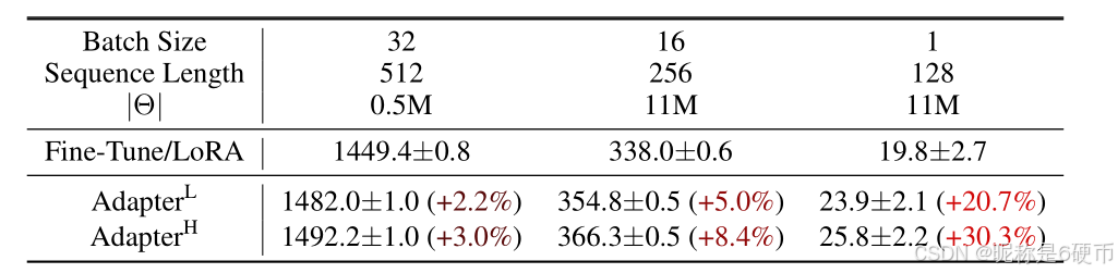
【翻译】表1:在GPT-2中等模型中单次前向传播的推理延迟,以毫秒为单位,对100次试验取平均值。我们使用NVIDIA Quadro RTX8000。"∣Θ∣\left|\Theta\right|∣Θ∣"表示适配器层中可训练参数的数量。AdapterL和AdapterH是适配器调优的两种变体,我们在第5.1节中描述。在在线、短序列长度场景中,适配器层引入的推理延迟可能很重要。详见附录B的完整研究。
【解析】推理延迟的实证测量结果。即使适配器层的参数量很小(通常远少于原模型的1%),但在在线推理场景中仍然会产生可观的延迟增加。这种延迟问题在短序列长度的应用中尤为突出,因为此时模型的计算主要集中在少量的token处理上,适配器层的顺序处理特性就成为了明显的瓶颈。
4 我们的方法
We describe the simple design of LoRA and its practical benefits. The principles outlined here apply to any dense layers in deep learning models, though we only focus on certain weights in Transformer language models in our experiments as the motivating use case.
【翻译】我们描述了LoRA的简单设计及其实际优势。这里概述的原理适用于深度学习模型中的任何密集层,尽管在我们的实验中,我们只专注于Transformer语言模型中的某些权重作为激励性用例。
4.1 低秩参数化更新矩阵
A neural network contains many dense layers which perform matrix multiplication. The weight matrices in these layers typically have full-rank. When adapting to a specific task, Aghajanyan et al. (2020) shows that the pre-trained language models have a low “instrisic dimension” and can still learn efficiently despite a random projection to a smaller subspace. Inspired by this, we hypothesize the updates to the weights also have a low “intrinsic rank” during adaptation. For a pre-trained weight matrix $ W_{0} \in\mathbb{R}^{{d}\times x}$, we constrain its update by representing the latter with a low-rank decomposition W0+ΔW=W0+BAW_{0}+\Delta W=W_{0}+B AW0+ΔW=W0+BA , where B∈Rd×r,A∈Rr×k{\boldsymbol B}\in\mathbb{R}^{{d}\times r}, {\boldsymbol A}\in\mathbb{R}^{r\times {{k}}}B∈Rd×r,A∈Rr×k , and the rank r≪min(d,k)r\ll\operatorname*{min}(d,k)r≪min(d,k) . During training, W0W_{0}W0 is frozen and does not receive gradient updates, while AAA and BBB contain trainable parameters. Note both W0W_{0}W0 and ΔW=BA\Delta W=B AΔW=BA are multiplied with the same input, and their respective output vectors are summed coordinate-wise. For h=W0xh=W_{0}xh=W0x , our modified forward pass yields:
h=W0x+ΔWx=W0x+BAxh=W_{0}x+\Delta W x=W_{0}x+B A x h=W0x+ΔWx=W0x+BAx
We illustrate our reparametrization in Figure 1. We use a random Gaussian initialization for AAA and zero for BBB , so ΔW=BA\Delta W=B AΔW=BA is zero at the beginning of training. We then scale ΔWx\Delta W xΔWx by αr\textstyle{\frac{\alpha}{r}}rα , where α\alphaα is a constant in rrr . When optimizing with Adam, tuning α\alphaα is roughly the same as tuning the learning rate if we scale the initialization appropriately. As a result, we simply set α\alphaα to the first rrr we try and do not tune it. This scaling helps to reduce the need to retune hyperparameters when we vary rrr (Yang & Hu, 2021).
【翻译】神经网络包含许多执行矩阵乘法的密集层。这些层中的权重矩阵通常具有满秩。当适应特定任务时,Aghajanyan等人(2020)表明预训练语言模型具有低"内在维度",即使通过随机投影到更小的子空间,仍然可以高效学习。受此启发,我们假设在适应过程中权重的更新也具有低"内在秩"。对于预训练权重矩阵W0∈Rd×kW_{0} \in\mathbb{R}^{{d}\times k}W0∈Rd×k,我们通过用低秩分解W0+ΔW=W0+BAW_{0}+\Delta W=W_{0}+BAW0+ΔW=W0+BA来表示后者,从而约束其更新,其中B∈Rd×r,A∈Rr×k{\boldsymbol B}\in\mathbb{R}^{{d}\times r}, {\boldsymbol A}\in\mathbb{R}^{r\times {{k}}}B∈Rd×r,A∈Rr×k,且秩r≪min(d,k)r\ll\operatorname*{min}(d,k)r≪min(d,k)。在训练期间,W0W_{0}W0被冻结且不接收梯度更新,而AAA和BBB包含可训练参数。注意W0W_{0}W0和ΔW=BA\Delta W=BAΔW=BA都与相同的输入相乘,它们各自的输出向量按坐标求和。对于h=W0xh=W_{0}xh=W0x,我们修改的前向传播产生。我们在图1中说明了我们的重新参数化。我们对AAA使用随机高斯初始化,对BBB使用零初始化,因此ΔW=BA\Delta W=BAΔW=BA在训练开始时为零。然后我们用αr\textstyle{\frac{\alpha}{r}}rα缩放ΔWx\Delta WxΔWx,其中α\alphaα是rrr中的常数。当使用Adam优化时,如果我们适当地缩放初始化,调整α\alphaα大致相当于调整学习率。因此,我们简单地将α\alphaα设置为我们尝试的第一个rrr,并且不调整它。这种缩放有助于减少当我们改变rrr时重新调整超参数的需要(Yang & Hu, 2021)。
【解析】Aghajanyan的研究表明,预训练语言模型具有低内在维度的特性,这说明模型的核心能力实际上集中在一个相对较小的参数子空间中,即使我们随机地将模型投影到一个更小的空间,模型依然能够保持良好的学习能力。基于这个发现,LoRA提出了一个关键假设:在模型适应新任务的过程中,权重的更新变化量ΔW\Delta WΔW也应该具有低内在秩的特性。这个假设的核心思想是,我们不需要更新整个权重矩阵,只需要学习一个低秩的变化量就足够了。具体的技术实现是将权重更新ΔW\Delta WΔW分解为两个更小矩阵的乘积BABABA,其中BBB的维度是d×rd \times rd×r,AAA的维度是r×kr \times kr×k,而rrr是一个远小于ddd和kkk的数值。这样做的好处是大幅减少了需要训练的参数数量,因为原来需要d×kd \times kd×k个参数,现在只需要d×r+r×kd \times r + r \times kd×r+r×k个参数,当rrr很小时,参数量减少是非常显著的。在实际训练过程中,原始的预训练权重W0W_0W0保持完全冻结状态,不接收任何梯度更新,只有AAA和BBB这两个低秩矩阵参与训练。前向传播的计算过程是将原始权重的输出和低秩更新的输出直接相加,这种并行计算的方式确保了推理阶段不会引入额外的计算延迟。初始化策略也很重要:AAA矩阵使用随机高斯分布初始化,而BBB矩阵初始化为零矩阵,这样确保了ΔW=BA\Delta W = BAΔW=BA在训练开始时为零,模型从预训练状态开始逐步学习任务特定的调整。缩放因子αr\frac{\alpha}{r}rα的引入是为了稳定训练过程,它类似于学习率的作用,帮助控制权重更新的幅度,使得当我们改变秩rrr的值时,不需要重新调整其他超参数。
A Generalization of Full Fine-tuning. A more general form of fine-tuning allows the training of a subset of the pre-trained parameters. LoRA takes a step further and does not require the accumulated gradient update to weight matrices to have full-rank during adaptation. This means that when applying LoRA to all weight matrices and training all biases, we roughly recover the expressiveness of full fine-tuning by setting the LoRA rank rrr to the rank of the pre-trained weight matrices. In other words, as we increase the number of trainable parameters, training LoRA roughly converges to training the original model, while adapter-based methods converges to an MLP and prefix-based methods to a model that cannot take long input sequences.
【翻译】全微调的泛化。更一般的微调形式允许训练预训练参数的子集。LoRA更进一步,不要求在适应过程中权重矩阵的累积梯度更新具有满秩。这说明当将LoRA应用于所有权重矩阵并训练所有偏置时,通过将LoRA秩rrr设置为预训练权重矩阵的秩,我们大致恢复了全微调的表达能力。换句话说,随着我们增加可训练参数的数量,训练LoRA大致收敛到训练原始模型,而基于适配器的方法收敛到MLP,基于前缀的方法收敛到无法处理长输入序列的模型。
【解析】将LoRA应用到模型的所有权重矩阵并训练所有偏置参数时,通过调整秩参数rrr到与原始预训练权重矩阵相同的秩,实际上可以恢复接近全微调的表达能力。相比之下,适配器方法本质上是在网络中插入小型的多层感知机模块,无论如何调整参数数量,其表达能力都被限制在这些MLP结构内。而前缀调优方法由于需要占用输入序列的长度来容纳可训练的前缀标记,其处理长序列的能力天然受到限制,无法通过增加参数来解决这个根本性的架构约束。
No Additional Inference Latency. When deployed in production, we can explicitly compute and store W=W0+BAW=W_{0}+B AW=W0+BA and perform inference as usual. Note that both W0W_{0}W0 and BAB ABA are in Rd×k\mathbb{R}^{d\times k}Rd×k . When we need to switch to another downstream task, we can recover W0W_{0}W0 by subtracting BAB ABA and then adding a different B′A′B^{\prime}A^{\prime}B′A′ , a quick operation with very little memory overhead. Critically, this guarantees that we do not introduce any additional latency during inference compared to a fine-tuned model by construction.
【翻译】无额外推理延迟。在生产部署时,我们可以显式计算并存储W=W0+BAW=W_{0}+BAW=W0+BA,然后像往常一样执行推理。注意W0W_{0}W0和BABABA都在Rd×k\mathbb{R}^{d\times k}Rd×k中。当我们需要切换到另一个下游任务时,我们可以通过减去BABABA然后添加不同的B′A′B^{\prime}A^{\prime}B′A′来恢复W0W_{0}W0,这是一个快速操作,内存开销很小。关键的是,这保证了与微调模型相比,我们在推理期间不会引入任何额外的延迟。
【解析】LoRA在实际部署中的关键优势:零推理延迟开销。可以预先计算合并后的权重矩阵W=W0+BAW = W_0 + BAW=W0+BA,并将其存储为单一的权重矩阵。由于原始权重W0W_0W0和低秩更新BABABA都具有相同的维度d×kd \times kd×k,它们可以直接相加得到最终的权重矩阵。具体来说,先通过W0=W−BAW_0 = W - BAW0=W−BA恢复原始的预训练权重,然后加上新任务对应的低秩更新B′A′B'A'B′A′,得到Wnew=W0+B′A′W_{new} = W_0 + B'A'Wnew=W0+B′A′。这个过程只涉及矩阵的加减运算,计算复杂度很低,内存开销也很小。
4.2 将LoRA应用到Transformer
In principle, we can apply LoRA to any subset of weight matrices in a neural network to reduce the number of trainable parameters. In the Transformer architecture, there are four weight matrices in the self-attention module (Wq,Wk,Wv,Wo)(W_{q},W_{k},W_{v},W_{o})(Wq,Wk,Wv,Wo) and two in the MLP module. We treat WqW_{q}Wq (or WkW_{k}Wk , WvW_{v}Wv ) as a single matrix of dimension dmodel×dmodel{d_{m o d e l}}\times{d_{m o d e l}}dmodel×dmodel , even though the output dimension is usually sliced into attention heads. We limit our study to only adapting the attention weights for downstream tasks and freeze the MLP modules (so they are not trained in downstream tasks) both for simplicity and parameter-efficiency.We further study the effect on adapting different types of attention weight matrices in a Transformer in Section 7.1. We leave the empirical investigation of adapting the MLP layers, LayerNorm layers, and biases to a future work.
【翻译】原则上,我们可以将LoRA应用于神经网络中权重矩阵的任何子集以减少可训练参数的数量。在Transformer架构中,自注意力模块中有四个权重矩阵(Wq,Wk,Wv,Wo)(W_{q},W_{k},W_{v},W_{o})(Wq,Wk,Wv,Wo),MLP模块中有两个。我们将WqW_{q}Wq(或WkW_{k}Wk、WvW_{v}Wv)视为维度为dmodel×dmodel{d_{m o d e l}}\times{d_{m o d e l}}dmodel×dmodel的单一矩阵,尽管输出维度通常被切分为注意力头。为了简单性和参数效率,我们将研究限制为仅对下游任务的注意力权重进行适配,并冻结MLP模块(因此它们在下游任务中不被训练)。我们在第7.1节中进一步研究了在Transformer中适配不同类型注意力权重矩阵的影响。我们将对MLP层、LayerNorm层和偏置的适配的实证研究留给未来的工作。
【解析】Transformer架构包含多个权重矩阵,其中自注意力机制包含查询WqW_qWq、键WkW_kWk、值WvW_vWv和输出投影WoW_oWo四个权重矩阵,而前馈网络MLP模块通常包含两个线性变换矩阵。虽然在多头注意力机制中,这些权重矩阵的输出会被划分为多个注意力头,但LoRA将整个权重矩阵作为一个统一的dmodel×dmodel{d_{model}} \times {d_{model}}dmodel×dmodel维度矩阵来处理。作者选择只对注意力权重进行低秩适配而冻结MLP模块的策略基于两个考虑:计算简化和参数效率最大化。MLP层通常承担非线性变换和特征提取的功能,而注意力机制主要负责序列中不同位置间的信息交互,通过只适配注意力权重,LoRA能够有效地调整模型对不同位置信息的关注模式,这对于大多数下游任务的适配是充分的。
Practical Benefits and Limitations. The most significant benefit comes from the reduction in memory and storage usage. For a large Transformer trained with Adam, we reduce that VRAM usage by up to 2/32/32/3 if r≪dmodelr\ll d_{model}r≪dmodel as we do not need to store the optimizer states for the frozen parameters. On GPT-3 175B, we reduce the VRAM consumption during training from 1.2TB to 350GB. With r=4r=4r=4 and only the query and value projection matrices being adapted, the checkpoint size is reduced by roughly 10,000×10{,}000\times10,000× (from 350GB to 35MB). This allows us to train with significantly fewer GPUs and avoid I/O bottlenecks. Another benefit is that we can switch between tasks while deployed at a much lower cost by only swapping the LoRA weights as opposed to all the parameters. This allows for the creation of many customized models that can be swapped in and out on the fly on machines that store the pre-trained weights.
【翻译】实用优势和局限性。最显著的好处来自内存和存储使用的减少。对于使用Adam训练的大型Transformer,如果r≪dmodelr\ll d_{model}r≪dmodel,我们可以减少高达2/32/32/3的显存使用,因为我们不需要为冻结参数存储优化器状态。在GPT-3 175B上,我们将训练期间的显存消耗从1.2TB减少到350GB。当r=4r=4r=4且仅适配查询和值投影矩阵时,检查点大小减少了大约10,00010{,}00010,000倍(从350GB到35MB)。这使我们能够用显著更少的GPU进行训练并避免I/O瓶颈。另一个好处是,我们可以通过仅交换LoRA权重而不是所有参数,以更低的成本在部署时切换任务。这允许创建许多定制模型,可以在存储预训练权重的机器上即时交换进出。
LoRA also has its limitations. For example, it is not straightforward to batch inputs to different tasks with different AAA and BBB in a single forward pass, if one chooses to absorb AAA and BBB into WWW to eliminate additional inference latency. Though it is possible to not merge the weights and dynamically choose the LoRA modules to use for samples in a batch for scenarios where latency is not critical.
【翻译】LoRA也有其局限性。例如,如果选择将AAA和BBB吸收到WWW中以消除额外的推理延迟,则在单次前向传播中将不同任务的输入与不同的AAA和BBB进行批处理并不简单。尽管在延迟不关键的场景中,可以不合并权重并动态选择要用于批次中样本的LoRA模块。
【解析】作者也指出了LoRA方法的局限。将低秩矩阵AAA和BBB预先合并到原始权重WWW中形成W+BAW + BAW+BA时,虽然能够消除推理时的额外计算开销,但这种合并是固定的,即每个合并后的权重矩阵只能对应一个特定的任务。在需要同时处理多个不同任务的批处理场景中,由于每个任务可能需要不同的AAA和BBB矩阵,系统无法在单次前向传播中高效地处理这样的混合批次。解决方案是保持LoRA权重的独立性,在运行时根据输入样本的任务类型动态选择相应的LoRA模块进行计算,但这会引入额外的计算开销和延迟。
5 实证实验
We evaluate the downstream task performance of LoRA on RoBERTa (Liu et al., 2019), DeBERTa (He et al., 2021), and GPT-2 (Radford et al., b), before scaling up to GPT-3 175B (Brown et al., 2020). Our experiments cover a wide range of tasks, from natural language understanding (NLU) to generation (NLG). Specifically, we evaluate on the GLUE (Wang et al., 2019) benchmark for RoBERTa and DeBERTa. We follow the setup of Li & Liang (2021) on GPT-2 for a direct comparison and add WikiSQL (Zhong et al., 2017) (NL to SQL queries) and SAMSum (Gliwa et al., 2019) (conversation summarization) for large-scale experiments on GPT-3. See Appendix C for more details on the datasets we use. We use NVIDIA Tesla V100 for all experiments.
【翻译】我们在RoBERTa(Liu等人,2019)、DeBERTa(He等人,2021)和GPT-2(Radford等人,b)上评估LoRA的下游任务性能,然后扩展到GPT-3 175B(Brown等人,2020)。我们的实验涵盖了从自然语言理解(NLU)到生成(NLG)的广泛任务。具体来说,我们在GLUE(Wang等人,2019)基准上评估RoBERTa和DeBERTa。我们遵循Li & Liang(2021)在GPT-2上的设置进行直接比较,并添加WikiSQL(Zhong等人,2017)(自然语言到SQL查询)和SAMSum(Gliwa等人,2019)(对话摘要)用于GPT-3的大规模实验。有关我们使用的数据集的更多详细信息,请参见附录C。我们在所有实验中使用NVIDIA Tesla V100。
5.1 基线方法
To compare with other baselines broadly, we replicate the setups used by prior work and reuse their reported numbers whenever possible. This, however, means that some baselines might only appear in certain experiments.
【翻译】为了与其他基线进行广泛比较,我们复制了先前工作使用的设置,并尽可能重用他们报告的数字。然而,这意味着某些基线可能只出现在特定实验中。
Fine-Tuning (FT) is a common approach for adaptation. During fine-tuning, the model is initialized to the pre-trained weights and biases, and all model parameters undergo gradient updates.A simple variant is to update only some layers while freezing others. We include one such baseline reported in prior work (Li & Liang, 2021) on GPT-2, which adapts just the last two layers (FTTop2)(\mathbf{FT}^{\mathbf{Top}2})(FTTop2) .
【翻译】微调(FT)是一种常见的适应方法。在微调过程中,模型被初始化为预训练的权重和偏置,所有模型参数都经历梯度更新。一个简单的变体是只更新某些层而冻结其他层。我们包括了先前工作(Li & Liang, 2021)在GPT-2上报告的一个这样的基线,它只适应最后两层(FTTop2)(\mathbf{FT}^{\mathbf{Top}2})(FTTop2)。
Table 2: RoBERTabase\mathrm{RoBERTa_{base}}RoBERTabase , RoBERTalarge\mathrm{RoBERTa_{large}}RoBERTalarge , and DeBERTaXXL\mathrm{DeBERTa_{XXL}}DeBERTaXXL with different adaptation methods on the GLUE benchmark. We report the overall (matched and mismatched) accuracy for MNLI, Matthew’s correlation for CoLA, Pearson correlation for STS-B, and accuracy for other tasks. Higher is better for all metrics. * indicates numbers published in prior works. †\dagger† indicates runs configured in a setup similar to Houlsby et al. (2019) for a fair comparison.
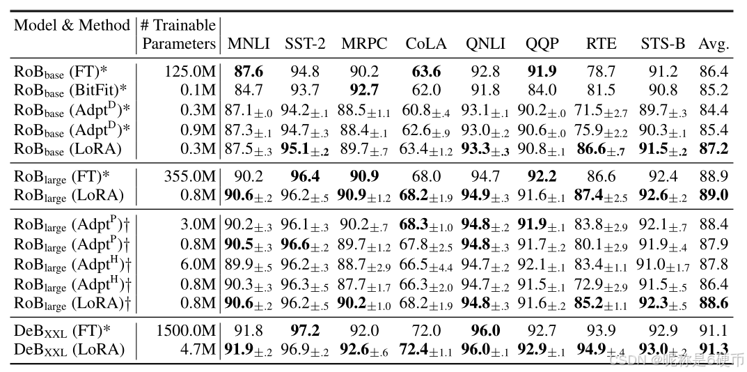
【翻译】表2:RoBERTabase\mathrm{RoBERTa_{base}}RoBERTabase、RoBERTalarge\mathrm{RoBERTa_{large}}RoBERTalarge和DeBERTaXXL\mathrm{DeBERTa_{XXL}}DeBERTaXXL在GLUE基准测试上使用不同适应方法的结果。我们报告了MNLI的整体(匹配和不匹配)准确率、CoLA的马修相关性、STS-B的皮尔逊相关性,以及其他任务的准确率。所有指标都是越高越好。*表示先前工作中发表的数字。†\dagger†表示为了公平比较而配置成类似于Houlsby等人(2019)设置的运行。
Bias-only or BitFit is a baseline where we only train the bias vectors while freezing everything else.
Contemporarily, this baseline has also been studied by BitFit (Zaken et al., 2021).
【翻译】仅偏置或BitFit是一个基线方法,我们只训练偏置向量而冻结其他所有参数。同时期,这个基线方法也在BitFit(Zaken等人,2021)中得到了研究。
Prefix-embedding tuning (PreEmbed) inserts special tokens among the input tokens. These special tokens have trainable word embeddings and are generally not in the model’s vocabulary. Where to place such tokens can have an impact on performance. We focus on “prefixing”, which prepends such tokens to the prompt, and “infixing”, which appends to the prompt; both are discussed in Li & Liang (2021). We use lpl_{p}lp (resp. lil_{i}li ) denote the number of prefix (resp. infix) tokens. The number of trainable parameters is ∣Θ∣=dmodel×(lp+li)|\Theta|=d_{model}\times\left(l_{p}+l_{i}\right)∣Θ∣=dmodel×(lp+li) .
【翻译】前缀嵌入调优(PreEmbed)在输入标记中插入特殊标记。这些特殊标记具有可训练的词嵌入,通常不在模型的词汇表中。这些标记的放置位置会对性能产生影响。我们专注于"前缀化"(将这些标记添加到提示前面)和"中缀化"(将其添加到提示后面);两者都在Li & Liang(2021)中讨论过。我们使用lpl_{p}lp(和lil_{i}li)分别表示前缀(和中缀)标记的数量。可训练参数的数量为∣Θ∣=dmodel×(lp+li)|\Theta|=d_{model}\times\left(l_{p}+l_{i}\right)∣Θ∣=dmodel×(lp+li)。
Prefix-layer tuning (PreLayer) is an extension to prefix-embedding tuning. Instead of just learning the word embeddings (or equivalently, the activations after the embedding layer) for some special tokens, we learn the activations after every Transformer layer. The activations computed from previous layers are simply replaced by trainable ones. The resulting number of trainable parameters is ∣Θ∣=L×dmodel×(lp+li)|\Theta|=L\times d_{m o d e l}\times\left(l_{p}+l_{i}\right)∣Θ∣=L×dmodel×(lp+li) , where LLL is the number of Transformer layers.
【翻译】前缀层调优(PreLayer)是前缀嵌入调优的扩展。我们不是仅仅学习某些特殊标记的词嵌入(或等价地,嵌入层后的激活),而是学习每个Transformer层后的激活。从前面层计算出的激活被可训练的激活简单地替换。由此产生的可训练参数数量为∣Θ∣=L×dmodel×(lp+li)|\Theta|=L\times d_{m o d e l}\times\left(l_{p}+l_{i}\right)∣Θ∣=L×dmodel×(lp+li),其中LLL是Transformer层的数量。
Adapter tuning as proposed in Houlsby et al. (2019) inserts adapter layers between the selfattention module (and the MLP module) and the subsequent residual connection. There are two fully connected layers with biases in an adapter layer with a nonlinearity in between. We call this original design AdapterHAdapter^{H}AdapterH. Recently, Lin et al. (2020) proposed a more efficient design with the adapter layer applied only after the MLP module and after a LayerNorm. We call it AdapterLAdapter^{L}AdapterL . This is very similar to another deign proposed in Pfeiffer et al. (2021), which we call AdapterPAdapter^{P}AdapterP . We also include another baseline call AdapterDrop (Ruicklé et al., 2020) which drops some adapter layers for greater efficiency (AdapterDAdapter^{D}AdapterD). We cite numbers from prior works whenever possible to maximize the number of baselines we compare with; they are in rows with an asterisk (∗)({}^{*})(∗) in the first column. In all cases, we have ∣Θ∣=L^Adpt×(2×dmodel×r+r+dmodel)+2×L^LN×dmodel|\Theta|=\hat{L}_{A d p t}\times(2\times d_{m o d e l}\times r+r+d_{m o d e l})+2\times\hat{L}_{L N}\times d_{m o d e l}∣Θ∣=L^Adpt×(2×dmodel×r+r+dmodel)+2×L^LN×dmodel where L^Adpt\hat{L}_{A d p t}L^Adpt is the number of adapter layers and L^LN\hat{L}_{L N}L^LN the number of trainable LayerNorms (e.g., in AdapterLAdapter^{L}AdapterL).
【翻译】Houlsby等人(2019)提出的适配器调优在自注意力模块(和MLP模块)与后续残差连接之间插入适配器层。适配器层中有两个带偏置的全连接层,中间有一个非线性激活。我们称这个原始设计为AdapterHAdapter^{H}AdapterH。最近,Lin等人(2020)提出了一个更高效的设计,适配器层仅应用在MLP模块之后和LayerNorm之后。我们称之为AdapterLAdapter^{L}AdapterL。这与Pfeiffer等人(2021)提出的另一个设计非常相似,我们称之为AdapterPAdapter^{P}AdapterP。我们还包括另一个称为AdapterDrop(Ruicklé等人,2020)的基线,它丢弃一些适配器层以获得更高的效率(AdapterDAdapter^{D}AdapterD)。我们尽可能引用先前工作的数字,以最大化我们比较的基线数量;它们在第一列带有星号(∗)({}^{*})(∗)的行中。在所有情况下,我们有∣Θ∣=L^Adpt×(2×dmodel×r+r+dmodel)+2×L^LN×dmodel|\Theta|=\hat{L}_{A d p t}\times(2\times d_{m o d e l}\times r+r+d_{m o d e l})+2\times\hat{L}_{L N}\times d_{m o d e l}∣Θ∣=L^Adpt×(2×dmodel×r+r+dmodel)+2×L^LN×dmodel,其中L^Adpt\hat{L}_{A d p t}L^Adpt是适配器层的数量,L^LN\hat{L}_{L N}L^LN是可训练LayerNorm的数量(例如,在AdapterLAdapter^{L}AdapterL中)。
LoRA adds trainable pairs of rank decomposition matrices in parallel to existing weight matrices. As mentioned in Section 4.2, we only apply LoRA to WqW_{q}Wq and WvW_{v}Wv in most experiments for simplicity. The number of trainable parameters is determined by the rank rrr and the shape of the original weights: ∣Θ∣=2×L^LoRA×dmodel×r|\Theta|=2\times\hat{L}_{L o R A}\times d_{m o d e l}\times r∣Θ∣=2×L^LoRA×dmodel×r , where L^LoRA\hat{L}_{L o R A}L^LoRA is the number of weight matrices we apply LoRA to.
【翻译】LoRA在现有权重矩阵的基础上并行添加可训练的秩分解矩阵对。如第4.2节所述,为了简化,我们在大多数实验中只将LoRA应用于WqW_{q}Wq和WvW_{v}Wv。可训练参数的数量由秩rrr和原始权重的形状决定:∣Θ∣=2×L^LoRA×dmodel×r|\Theta|=2\times\hat{L}_{L o R A}\times d_{m o d e l}\times r∣Θ∣=2×L^LoRA×dmodel×r,其中L^LoRA\hat{L}_{L o R A}L^LoRA是我们应用LoRA的权重矩阵数量。
Table 3: GPT-2 medium (M) and large (L) with different adaptation methods on the E2E NLG Challenge. For all metrics, higher is better. LoRA outperforms several baselines with comparable or fewer trainable parameters. Confidence intervals are shown for experiments we ran. * indicates numbers published in prior works.
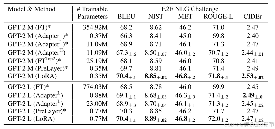
【翻译】表3:GPT-2 medium(M)和large(L)在E2E NLG Challenge上使用不同适应方法的结果。所有指标都是越高越好。LoRA在具有相当或更少可训练参数的情况下优于几个基线方法。置信区间显示为我们运行的实验。*表示先前工作中发表的数字。
5.2 RoBERTa Base/Large实验
RoBERTa (Liu et al., 2019) optimized the pre-training recipe originally proposed in BERT (Devlin et al., 2019a) and boosted the latter’s task performance without introducing many more trainable parameters. While RoBERTa has been overtaken by much larger models on NLP leaderboards such as the GLUE benchmark (Wang et al., 2019) in recent years, it remains a competitive and popular pre-trained model for its size among practitioners. We take the pre-trained RoBERTa base (125M) and RoBERTa large (355M) from the HuggingFace Transformers library (Wolf et al., 2020) and evaluate the performance of different efficient adaptation approaches on tasks from the GLUE benchmark. We also replicate Houlsby et al. (2019) and Pfeiffer et al. (2021) according to their setup. To ensure a fair comparison, we make two crucial changes to how we evaluate LoRA when comparing with adapters. First, we use the same batch size for all tasks and use a sequence length of 128 to match the adapter baselines. Second, we initialize the model to the pre-trained model for MRPC, RTE, and STS-B, not a model already adapted to MNLI like the fine-tuning baseline. Runs following this more restricted setup from Houlsby et al. (2019) are labeled with †\dagger† . The result is presented in Table 2 (Top Three Sections). See Section D.1 for details on the hyperparameters used.
【翻译】RoBERTa(Liu等人,2019)优化了BERT(Devlin等人,2019a)最初提出的预训练配方,在不引入过多可训练参数的情况下提升了后者的任务性能。虽然近年来RoBERTa在NLP排行榜(如GLUE基准(Wang等人,2019))上已被更大的模型超越,但在同等规模的模型中,它仍然是实践者中具有竞争力且流行的预训练模型。我们从HuggingFace Transformers库(Wolf等人,2020)中获取预训练的RoBERTa base(125M)和RoBERTa large(355M),并在GLUE基准的任务上评估不同高效适应方法的性能。我们还根据Houlsby等人(2019)和Pfeiffer等人(2021)的设置复制了他们的实验。为了确保公平比较,我们在将LoRA与适配器进行比较时对LoRA的评估方式做了两个关键改变。首先,我们对所有任务使用相同的批量大小,并使用序列长度128来匹配适配器基线。其次,对于MRPC、RTE和STS-B,我们将模型初始化为预训练模型,而不是像微调基线那样使用已经适应MNLI的模型。遵循Houlsby等人(2019)这种更严格设置的运行用†\dagger†标记。结果呈现在表2(前三个部分)中。有关所使用超参数的详细信息,请参见第D.1节。
5.3 DeBERTa XXL实验
DeBERTa (He et al., 2021) is a more recent variant of BERT that is trained on a much larger scale and performs very competitively on benchmarks such as GLUE (Wang et al., 2019) and SuperGLUE (Wang et al., 2020). We evaluate if LoRA can still match the performance of a fully fine-tuned DeBERTa XXL (1.5B) on GLUE. The result is presented in Table 2 (Bottom Section). See Section D.2 for details on the hyperparameters used.
【翻译】DeBERTa(He等人,2021)是BERT的一个更新变体,它在更大规模上进行训练,在GLUE(Wang等人,2019)和SuperGLUE(Wang等人,2020)等基准测试上表现非常具有竞争力。我们评估LoRA是否仍能在GLUE上匹配完全微调的DeBERTa XXL(1.5B)的性能。结果呈现在表2(底部部分)中。有关所使用超参数的详细信息,请参见第D.2节。
5.4 GPT-2 中型/大型模型实验
Having shown that LoRA can be a competitive alternative to full fine-tuning on NLU, we hope to answer if LoRA still prevails on NLG models, such as GPT-2 medium and large (Radford et al., b). We keep our setup as close as possible to Li & Liang (2021) for a direct comparison. Due to space constraint, we only present our result on E2E NLG Challenge (Table 3) in this section. See Section F.1 for results on WebNLG (Gardent et al., 2017) and DART (Nan et al., 2020). We include a list of the hyperparameters used in Section D.3.
【翻译】在证明了LoRA可以作为NLU全参数微调的竞争性替代方案后,我们希望回答LoRA是否在NLG模型(如GPT-2 medium和large(Radford等人,b))上仍然占优。为了直接比较,我们尽可能保持与Li & Liang(2021)相同的设置。由于篇幅限制,本节中我们只展示在E2E NLG Challenge(表3)上的结果。WebNLG(Gardent等人,2017)和DART(Nan等人,2020)的结果请参见第F.1节。我们在第D.3节中包含了所使用的超参数列表。
Table 4: Performance of different adaptation methods on GPT-3 175B. We report the logical form validation accuracy on WikiSQL, validation accuracy on MultiNLI-matched, and Rouge-1/2/L on SAMSum. LoRA performs better than prior approaches, including full fine-tuning. The results on WikiSQL have a fluctuation around ±0.5%\pm0.5\%±0.5% , MNLI-m around ±0.1%\pm0.1\%±0.1% , and SAMSum around ±0.2/±0.2/±0.1\pm0.2/\pm0.2/\pm0.1±0.2/±0.2/±0.1 for the three metrics.
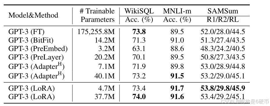
【翻译】表4:不同适应方法在GPT-3 175B上的性能。我们报告了WikiSQL上的逻辑形式验证准确率、MultiNLI-matched上的验证准确率,以及SAMSum上的Rouge-1/2/L指标。LoRA的性能优于之前的方法,包括全参数微调。WikiSQL上的结果波动约为±0.5%\pm0.5\%±0.5%,MNLI-m约为±0.1%\pm0.1\%±0.1%,SAMSum在三个指标上分别约为±0.2/±0.2/±0.1\pm0.2/\pm0.2/\pm0.1±0.2/±0.2/±0.1。
5.5 扩展到GPT-3 175B
As a final stress test for LoRA, we scale up to GPT-3 with 175 billion parameters. Due to the high training cost, we only report the typical standard deviation for a given task over random seeds, as opposed to providing one for every entry. See Section D.4 for details on the hyperparameters used.
【翻译】作为LoRA的最终压力测试,我们扩展到拥有1750亿参数的GPT-3。由于训练成本很高,我们只报告给定任务在随机种子上的典型标准偏差,而不是为每个条目提供一个。有关所使用超参数的详细信息,请参见第D.4节。
As shown in Table 4, LoRA matches or exceeds the fine-tuning baseline on all three datasets. Note that not all methods benefit monotonically from having more trainable parameters, as shown in Figure 2. We observe a significant performance drop when we use more than 256 special tokens for prefix-embedding tuning or more than 32 special tokens for prefix-layer tuning. This corroborates similar observations in Li & Liang (2021). While a thorough investigation into this phenomenon is out-of-scope for this work, we suspect that having more special tokens causes the input distribution to shift further away from the pre-training data distribution. Separately, we investigate the performance of different adaptation approaches in the low-data regime in Section F.3.
【翻译】如表4所示,LoRA在所有三个数据集上都匹配或超过了微调基线。请注意,并非所有方法都能从拥有更多可训练参数中单调受益,如图2所示。我们观察到,当我们在前缀嵌入调优中使用超过256个特殊标记或在前缀层调优中使用超过32个特殊标记时,性能显著下降。这证实了Li & Liang(2021)中的类似观察。虽然对这一现象的彻底调查超出了本工作的范围,但我们怀疑拥有更多特殊标记会导致输入分布进一步偏离预训练数据分布。另外,我们在第F.3节中调查了不同适应方法在低数据环境下的性能。
Figure 2: GPT-3 175B validation accuracy vs. number of trainable parameters of several adaptation methods on WikiSQL and MNLI-matched. LoRA exhibits better scalability and task performance. See Section F.2 for more details on the plotted data points.
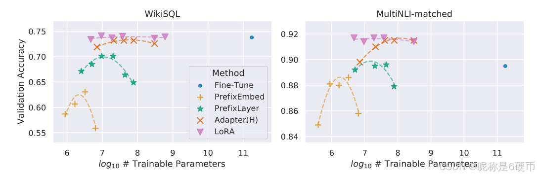
【翻译】图2:几种适应方法在WikiSQL和MNLI-matched上的GPT-3 175B验证准确率与可训练参数数量的关系。LoRA表现出更好的可扩展性和任务性能。有关绘制数据点的更多详细信息,请参见第F.2节。
6 相关工作
Transformer Language Models. Transformer (Vaswani et al., 2017) is a sequence-to-sequence architecture that makes heavy use of self-attention. Radford et al. (a) applied it to autoregressive language modeling by using a stack of Transformer decoders. Since then, Transformer-based language models have dominated NLP, achieving the state-of-the-art in many tasks. A new paradigm emerged with BERT (Devlin et al., 2019b) and GPT-2 (Radford et al., b) – both are large Transformer language models trained on a large amount of text – where fine-tuning on task-specific data after pretraining on general domain data provides a significant performance gain compared to training on task-specific data directly. Training larger Transformers generally results in better performance and remains an active research direction. GPT-3 (Brown et al., 2020) is the largest single Transformer language model trained to-date with 175B parameters.
【翻译】Transformer语言模型。Transformer(Vaswani等人,2017)是一种大量使用自注意力机制的序列到序列架构。Radford等人(a)通过使用Transformer解码器堆栈将其应用于自回归语言建模。从那时起,基于Transformer的语言模型在NLP领域占据主导地位,在许多任务上达到了最先进的水平。BERT(Devlin等人,2019b)和GPT-2(Radford等人,b)出现了一种新的范式——两者都是在大量文本上训练的大型Transformer语言模型——在通用领域数据上预训练后对特定任务数据进行微调,与直接在特定任务数据上训练相比,提供了显著的性能提升。训练更大的Transformer通常会带来更好的性能,这仍然是一个活跃的研究方向。GPT-3(Brown等人,2020)是迄今为止训练的最大的单一Transformer语言模型,拥有1750亿参数。
Prompt Engineering and Fine-Tuning. While GPT-3 175B can adapt its behavior with just a few additional training examples, the result depends heavily on the input prompt (Brown et al., 2020). This necessitates an empirical art of composing and formatting the prompt to maximize a model’s performance on a desired task, which is known as prompt engineering or prompt hacking. Fine-tuning retrains a model pre-trained on general domains to a specific task Devlin et al. (2019b); Radford et al. (a). Variants of it include learning just a subset of the parameters Devlin et al. (2019b); Collobert & Weston (2008), yet practitioners often retrain all of them to maximize the downstream performance. However, the enormity of GPT-3 175B makes it challenging to perform fine-tuning in the usual way due to the large checkpoint it produces and the high hardware barrier to entry since it has the same memory footprint as pre-training.
【翻译】提示工程和微调。虽然GPT-3 175B可以仅用少数额外的训练示例来调整其行为,但结果严重依赖于输入提示(Brown等人,2020)。这需要一种组合和格式化提示的经验艺术,以最大化模型在期望任务上的性能,这被称为提示工程或提示黑客。微调将在通用领域上预训练的模型重新训练到特定任务上(Devlin等人,2019b;Radford等人,a)。其变体包括仅学习参数的子集(Devlin等人,2019b;Collobert & Weston,2008),然而实践者通常重新训练所有参数以最大化下游性能。然而,GPT-3 175B的巨大规模使得以通常方式进行微调具有挑战性,因为它产生大型检查点,并且由于其与预训练相同的内存占用而具有较高的硬件门槛。
Parameter-Efficient Adaptation. Many have proposed inserting adapter layers between existing layers in a neural network (Houlsby et al., 2019; Rebuffi et al., 2017; Lin et al., 2020). Our method uses a similar bottleneck structure to impose a low-rank constraint on the weight updates. The key functional difference is that our learned weights can be merged with the main weights during inference, thus not introducing any latency, which is not the case for the adapter layers (Section 3). A comtenporary extension of adapter is COMPACTER (Mahabadi et al., 2021), which essentially parametrizes the adapter layers using Kronecker products with some predetermined weight sharing scheme. Similarly, combining LoRA with other tensor product-based methods could potentially improve its parameter efficiency, which we leave to future work. More recently, many proposed optimizing the input word embeddings in lieu of fine-tuning, akin to a continuous and differentiable generalization of prompt engineering (Li & Liang, 2021; Lester et al., 2021; Hambardzumyan et al., 2020; Liu et al., 2021). We include comparisons with Li & Liang (2021) in our experiment section. However, this line of works can only scale up by using more special tokens in the prompt, which take up available sequence length for task tokens when positional embeddings are learned.
【翻译】参数高效适应。许多人提出在神经网络的现有层之间插入适配器层(Houlsby等人,2019;Rebuffi等人,2017;Lin等人,2020)。我们的方法使用类似的瓶颈结构对权重更新施加低秩约束。关键的功能差异是我们学习的权重可以在推理期间与主要权重合并,因此不会引入任何延迟,而适配器层则不是这种情况(第3节)。适配器的一个当代扩展是COMPACTER(Mahabadi等人,2021),它本质上使用Kronecker乘积和一些预定义的权重共享方案来参数化适配器层。类似地,将LoRA与其他基于张量乘积的方法结合可能会提高其参数效率,我们将此留给未来的工作。最近,许多人提出优化输入词嵌入来代替微调,类似于提示工程的连续和可微分推广(Li & Liang,2021;Lester等人,2021;Hambardzumyan等人,2020;Liu等人,2021)。我们在实验部分包含了与Li & Liang(2021)的比较。然而,这类工作只能通过在提示中使用更多特殊标记来扩展,当学习位置嵌入时,这会占用任务标记的可用序列长度。
Low-Rank Structures in Deep Learning. Low-rank structure is very common in machine learning. A lot of machine learning problems have certain intrinsic low-rank structure (Li et al., 2016; Cai et al., 2010; Li et al., 2018b; Grasedyck et al., 2013). Moreover, it is known that for many deep learning tasks, especially those with a heavily over-parametrized neural network, the learned neural network will enjoy low-rank properties after training (Oymak et al., 2019). Some prior works even explicitly impose the low-rank constraint when training the original neural network (Sainath et al., 2013; Povey et al., 2018; Zhang et al., 2014; Jaderberg et al., 2014; Zhao et al., 2016; Khodak et al., 2021; Denil et al., 2014); however, to the best of our knowledge, none of these works considers low-rank update to a frozen model for adaptation to downstream tasks. In theory literature, it is known that neural networks outperform other classical learning methods, including the corresponding (finite-width) neural tangent kernels (Allen-Zhu et al., 2019; Li & Liang, 2018) when the underlying concept class has certain low-rank structure (Ghorbani et al., 2020; Allen-Zhu & Li, 2019; Allen-Zhu & Li, 2020a). Another theoretical result in Allen-Zhu & Li (2020b) suggests that low-rank adaptations can be useful for adversarial training. In sum, we believe that our proposed low-rank adaptation update is well-motivated by the literature.
【翻译】深度学习中的低秩结构。低秩结构在机器学习中非常常见。许多机器学习问题具有某种内在的低秩结构(Li等人,2016;Cai等人,2010;Li等人,2018b;Grasedyck等人,2013)。此外,众所周知,对于许多深度学习任务,特别是那些具有严重过度参数化神经网络的任务,学习到的神经网络在训练后会享有低秩特性(Oymak等人,2019)。一些先前的工作甚至在训练原始神经网络时明确施加低秩约束(Sainath等人,2013;Povey等人,2018;Zhang等人,2014;Jaderberg等人,2014;Zhao等人,2016;Khodak等人,2021;Denil等人,2014);然而,据我们所知,这些工作中没有一个考虑对冻结模型进行低秩更新以适应下游任务。在理论文献中,众所周知,当底层概念类具有某种低秩结构时,神经网络的性能优于其他经典学习方法,包括相应的(有限宽度)神经切线核(Allen-Zhu等人,2019;Li & Liang,2018)(Ghorbani等人,2020;Allen-Zhu & Li,2019;Allen-Zhu & Li,2020a)。Allen-Zhu & Li(2020b)的另一个理论结果表明,低秩适应可能对对抗训练有用。总之,我们认为我们提出的低秩适应更新在文献中是有充分动机的。
7 理解低秩更新
Given the empirical advantage of LoRA, we hope to further explain the properties of the low-rank adaptation learned from downstream tasks. Note that the low-rank structure not only lowers the hardware barrier to entry which allows us to run multiple experiments in parallel, but also gives better interpretability of how the update weights are correlated with the pre-trained weights. We focus our study on GPT-3 175B, where we achieved the largest reduction of trainable parameters (up to 10,000×)10{,}000{\times})10,000×) without adversely affecting task performances.
【翻译】鉴于LoRA的经验优势,我们希望进一步解释从下游任务中学习到的低秩适应的特性。请注意,低秩结构不仅降低了硬件门槛,使我们能够并行运行多个实验,还提供了更好的可解释性,说明更新权重如何与预训练权重相关联。我们将研究重点放在GPT-3 175B上,在该模型上我们实现了最大的可训练参数减少(高达10,000×10{,}000{\times}10,000×),而不会对任务性能产生不利影响。
We perform a sequence of empirical studies to answer the following questions: 1) Given a parameter budget constraint, which subset of weight matrices in a pre-trained Transformer should we adapt to maximize downstream performance? 2) Is the “optimal” adaptation matrix ΔW\Delta WΔW really rankdeficient? If so, what is a good rank to use in practice? 3) What is the connection between ΔW\Delta WΔW and W?W?W? Does ΔW\Delta WΔW highly correlate with W ? How large is ΔW\Delta WΔW comparing to W?W?W?
【翻译】我们进行一系列经验研究来回答以下问题:1)在参数预算约束下,我们应该适应预训练Transformer中的哪个权重矩阵子集以最大化下游性能?2)“最优"适应矩阵ΔW\Delta WΔW真的是秩不足的吗?如果是,在实践中使用什么秩比较好?3)ΔW\Delta WΔW和WWW之间的联系是什么?ΔW\Delta WΔW与W高度相关吗?与WWW相比,ΔW\Delta WΔW有多"大”?
We believe that our answers to question (2) and (3) shed light on the fundamental principles of using pre-trained language models for downstream tasks, which is a critical topic in NLP.
【翻译】我们相信我们对问题(2)和(3)的回答阐明了将预训练语言模型用于下游任务的基本原理,这是NLP中的一个关键话题。
7.1 我们应该将LORA应用到TRANSFORMER中的哪些权重矩阵?
Given a limited parameter budget, which types of weights should we adapt with LoRA to obtain the best performance on downstream tasks? As mentioned in Section 4.2, we only consider weight matrices in the self-attention module. We set a parameter budget of 18M (roughly 35MB if stored in FP16) on GPT-3 175B, which corresponds to r=8r=8r=8 if we adapt one type of attention weights or r=4r=4r=4 if we adapt two types, for all 96 layers. The result is presented in Table 5.
【翻译】在有限的参数预算下,我们应该使用LoRA适应哪些类型的权重以在下游任务上获得最佳性能?如第4.2节所述,我们只考虑自注意力模块中的权重矩阵。我们在GPT-3 175B上设置了18M的参数预算(如果以FP16格式存储,大约为35MB),对于所有96层,如果我们适应一种类型的注意力权重,则对应r=8r=8r=8,如果我们适应两种类型,则对应r=4r=4r=4。结果在表5中呈现。
Table 5: Validation accuracy on WikiSQL and MultiNLI after applying LoRA to different types of attention weights in GPT-3, given the same number of trainable parameters. Adapting both WqW_{q}Wq and WvW_{v}Wv gives the best performance overall. We find the standard deviation across random seeds to be consistent for a given dataset, which we report in the first column.
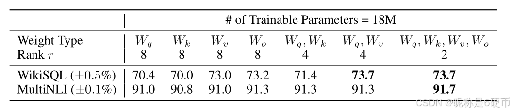
【翻译】表5:在给定相同数量的可训练参数下,将LoRA应用于GPT-3中不同类型注意力权重后在WikiSQL和MultiNLI上的验证准确率。同时适应WqW_{q}Wq和WvW_{v}Wv总体上给出了最佳性能。我们发现对于给定数据集,随机种子间的标准偏差是一致的,我们在第一列中报告了这一点。
Note that putting all the parameters in ΔWq\Delta W_{q}ΔWq or ΔWk\Delta W_{k}ΔWk results in significantly lower performance, while adapting both WqW_{q}Wq and WvW_{v}Wv yields the best result. This suggests that even a rank of four captures enough information in ΔW\Delta WΔW such that it is preferable to adapt more weight matrices than adapting a single type of weights with a larger rank.
【翻译】请注意,将所有参数放在ΔWq\Delta W_{q}ΔWq或ΔWk\Delta W_{k}ΔWk中会导致性能显著降低,而同时适应WqW_{q}Wq和WvW_{v}Wv产生最佳结果。这表明即使秩为4也能在ΔW\Delta WΔW中捕获足够的信息,因此适应更多权重矩阵比用更大的秩适应单一类型的权重更可取。
7.2 对于LoRA来说,最优秩rrr是多少?
We turn our attention to the effect of rank rrr on model performance. We adapt {Wq,Wv}\{W_{q},W_{v}\}{Wq,Wv} , {Wq,Wk,Wv,Wc}\{W_{q},W_{k},W_{v},W_{c}\}{Wq,Wk,Wv,Wc} , and just WqW_{q}Wq for a comparison.
【翻译】我们将注意力转向秩rrr对模型性能的影响。我们适应{Wq,Wv}\{W_{q},W_{v}\}{Wq,Wv}、{Wq,Wk,Wv,Wc}\{W_{q},W_{k},W_{v},W_{c}\}{Wq,Wk,Wv,Wc},以及仅WqW_{q}Wq进行比较。
Table 6: Validation accuracy on WikiSQL and MultiNLI with different rank rrr . To our surprise, a rank as small as one suffices for adapting both WqW_{q}Wq and WvW_{v}Wv on these datasets while training WqW_{q}Wq alone needs a larger rrr . We conduct a similar experiment on GPT-2 in Section H.2.
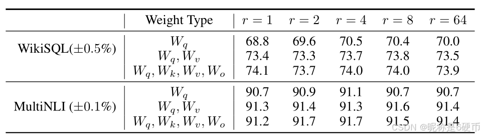
【翻译】表6:不同秩rrr下在WikiSQL和MultiNLI上的验证准确率。令我们惊讶的是,在这些数据集上,秩小到1就足以同时适应WqW_{q}Wq和WvW_{v}Wv,而单独训练WqW_{q}Wq需要更大的rrr。我们在第H.2节对GPT-2进行了类似的实验。
Table 6 shows that, surprisingly, LoRA already performs competitively with a very small rrr (more so for {Wq,Wv}\{W_{q},W_{v}\}{Wq,Wv} than just Wq,W_{q},Wq, ). This suggests the update matrix ΔW\Delta WΔW could have a very small “intrinsic rank”. To further support this finding, we check the overlap of the subspaces learned by different choices of rrr and by different random seeds. We argue that increasing rrr does not cover a more meaningful subspace, which suggests that a low-rank adaptation matrix is sufficient.
【翻译】表6显示,令人惊讶的是,LoRA在非常小的rrr下就已经表现出竞争力(对于{Wq,Wv}\{W_{q},W_{v}\}{Wq,Wv}比仅WqW_{q}Wq更是如此)。这表明更新矩阵ΔW\Delta WΔW可能具有非常小的"内在秩"。为了进一步支持这一发现,我们检查了不同rrr选择和不同随机种子学习到的子空间的重叠。我们认为增加rrr并不能覆盖更有意义的子空间,这表明低秩适应矩阵是足够的。
Subspace similarity between different rrr . Given Ar=8A_{r=8}Ar=8 and Ar=64A_{r=64}Ar=64 which are the learned adaptation matrices with rank r=8r=8r=8 and 64 using the same pre-trained model, we perform singular value decomposition and obtain the right-singular unitary matrices UAr=8U_{A_{r=8}}UAr=8 and UAr=64U_{A_{r=64}}UAr=64 . We hope to answer: how much of the subspace spanned by the top iii singular vectors in UAr=8U_{A_{r=8}}UAr=8 (for 1≤i≤81\leq i\leq81≤i≤8 ) is contained in the subspace spanned by top jjj singular vectors of UAr=64U_{A_{r=64}}UAr=64 (for 1≤j≤64)1\leq j\leq64)1≤j≤64) ? We measure this quantity with a normalized subspace similarity based on the Grassmann distance (See Appendix G for a more formal discussion)
【翻译】不同rrr之间的子空间相似性。给定Ar=8A_{r=8}Ar=8和Ar=64A_{r=64}Ar=64,它们是使用相同预训练模型学习到的秩为r=8r=8r=8和64的适应矩阵,我们执行奇异值分解并获得右奇异酉矩阵UAr=8U_{A_{r=8}}UAr=8和UAr=64U_{A_{r=64}}UAr=64。我们希望回答:UAr=8U_{A_{r=8}}UAr=8中前iii个奇异向量张成的子空间(对于1≤i≤81\leq i\leq81≤i≤8)有多少包含在UAr=64U_{A_{r=64}}UAr=64的前jjj个奇异向量张成的子空间中(对于1≤j≤641\leq j\leq641≤j≤64)?我们使用基于Grassmann距离的归一化子空间相似性来测量这个量(更正式的讨论见附录G)
ϕ(Ar=8,Ar=64,i,j)=∣∣UAr=8i⊤UAr=64j∣∣F2min(i,j)∈[0,1]\phi(A_{r=8},A_{r=64},i,j)=\frac{||U_{A_{r=8}}^{i\top}U_{A_{r=64}}^{j}||_{F}^{2}}{\operatorname*{min}(i,j)}\in[0,1] ϕ(Ar=8,Ar=64,i,j)=min(i,j)∣∣UAr=8i⊤UAr=64j∣∣F2∈[0,1]
where UAr=8iU_{A_{r=8}}^{i}UAr=8i represents the columns of UAr=8U_{A_{r=8}}UAr=8 corresponding to the top- iii singular vectors.
【翻译】其中UAr=8iU_{A_{r=8}}^{i}UAr=8i表示UAr=8U_{A_{r=8}}UAr=8中对应于前iii个奇异向量的列。
ϕ(⋅)\phi(\cdot)ϕ(⋅) has a range of [0,1][0,1][0,1] , where 1 represents a complete overlap of subspaces and 0 a complete separation. See Figure 3 for how ϕ\phiϕ changes as we vary iii and jjj . We only look at the 48th layer (out of 96) due to space constraint, but the conclusion holds for other layers as well, as shown in Section H.1.
【翻译】ϕ(⋅)\phi(\cdot)ϕ(⋅)的取值范围是[0,1][0,1][0,1],其中1表示子空间完全重叠,0表示完全分离。参见图3了解当我们改变iii和jjj时ϕ\phiϕ如何变化。由于空间限制,我们只查看第48层(共96层),但结论对其他层也成立,如第H.1节所示。
ϕ(Ar=64,Ar=8,i,j)\phi(A_{r=64},A_{r=8},i,j) ϕ(Ar=64,Ar=8,i,j)
Figure 3: Subspace similarity between column vectors of Ar=8A_{r=8}Ar=8 and Ar=64A_{r=64}Ar=64 for both ΔWq\Delta W_{q}ΔWq and ΔWv\Delta W_{v}ΔWv . The third and the fourth figures zoom in on the lower-left triangle in the first two figures. The top directions in r=8r=8r=8 are included in r=64r=64r=64 , and vice versa.
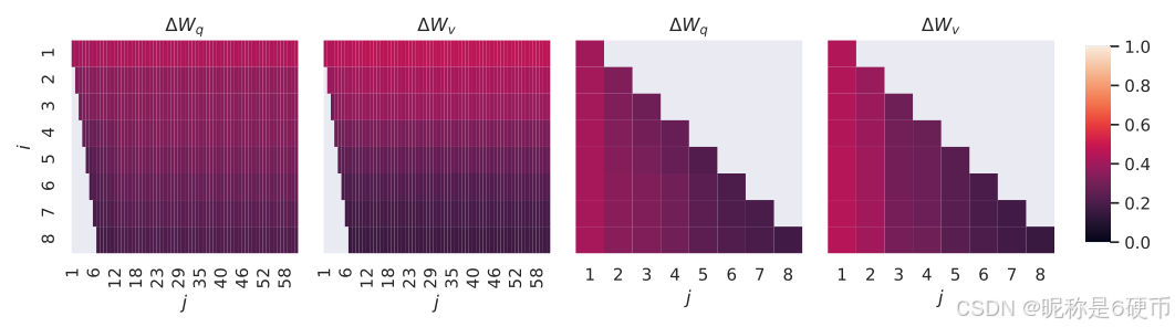
【翻译】图3:ΔWq\Delta W_{q}ΔWq和ΔWv\Delta W_{v}ΔWv的Ar=8A_{r=8}Ar=8和Ar=64A_{r=64}Ar=64列向量之间的子空间相似性。第三和第四个图放大了前两个图中的左下三角形。r=8r=8r=8中的顶部方向包含在r=64r=64r=64中,反之亦然。
We make an important observation from Figure 3.
【翻译】我们从图3中得出一个重要观察。
Directions corresponding to the top singular vector overlap significantly between Ar=8A_{r=8}Ar=8 and Ar=64A_{r=64}Ar=64 , while others do not. Specifically, ΔWv\Delta W_{v}ΔWv (resp. ΔWq)\Delta W_{q})ΔWq) ) of Ar=8A_{r=8}Ar=8 and ΔWv\Delta W_{v}ΔWv (resp. ΔWq,\Delta W_{q},ΔWq, ) of Ar=64A_{r=64}Ar=64 share a subspace of dimension 1 with normalized similarity >0.5>0.5>0.5 , providing an explanation of why r=1r=1r=1 performs quite well in our downstream tasks for GPT-3.
【翻译】对应于顶部奇异向量的方向在Ar=8A_{r=8}Ar=8和Ar=64A_{r=64}Ar=64之间显著重叠,而其他方向则不然。具体来说,Ar=8A_{r=8}Ar=8的ΔWv\Delta W_{v}ΔWv(分别是ΔWq\Delta W_{q}ΔWq)和Ar=64A_{r=64}Ar=64的ΔWv\Delta W_{v}ΔWv(分别是ΔWq\Delta W_{q}ΔWq)共享一个维度为1的子空间,其归一化相似性>0.5>0.5>0.5,这解释了为什么r=1r=1r=1在我们GPT-3的下游任务中表现相当好。
Since both Ar=8A_{r=8}Ar=8 and Ar=64A_{r=64}Ar=64 are learned using the same pre-trained model, Figure 3 indicates that the top singular-vector directions of Ar=8A_{r=8}Ar=8 and Ar=64A_{r=64}Ar=64 are the most useful, while other directions potentially contain mostly random noises accumulated during training. Hence, the adaptation matrix can indeed have a very low rank.
【翻译】由于Ar=8A_{r=8}Ar=8和Ar=64A_{r=64}Ar=64都是使用相同的预训练模型学习的,图3表明Ar=8A_{r=8}Ar=8和Ar=64A_{r=64}Ar=64的顶部奇异向量方向是最有用的,而其他方向可能主要包含训练过程中积累的随机噪声。因此,适应矩阵确实可以具有非常低的秩。
Subspace similarity between different random seeds. We further confirm this by plotting the normalized subspace similarity between two randomly seeded runs with r=64r=64r=64 , shown in Figure 4. ΔWq\Delta W_{q}ΔWq appears to have a higher “intrinsic rank” than ΔWv\Delta W_{v}ΔWv , since more common singular value directions are learned by both runs for ΔWq\Delta W_{q}ΔWq , which is in line with our empirical observation in Table 6. As a comparison, we also plot two random Gaussian matrices, which do not share any common singular value directions with each other.
【翻译】不同随机种子之间的子空间相似性。我们通过绘制两个随机种子运行(r=64r=64r=64)之间的归一化子空间相似性进一步确认了这一点,如图4所示。ΔWq\Delta W_{q}ΔWq似乎比ΔWv\Delta W_{v}ΔWv具有更高的"内在秩",因为两次运行都学到了ΔWq\Delta W_{q}ΔWq的更多共同奇异值方向,这与我们在表6中的经验观察一致。作为比较,我们还绘制了两个随机高斯矩阵,它们彼此之间不共享任何共同的奇异值方向。
7.3 适应矩阵 ∆W 与 WWW 的比较关系如何?
We further investigate the relationship between ΔW\Delta WΔW and WWW . In particular, does ΔW\Delta WΔW highly correlate with WWW ? (Or mathematically, is ΔW\Delta WΔW mostly contained in the top singular directions of W?W?W? ) Also, how “large” is ΔW\Delta WΔW comparing to its corresponding directions in $W ? This can shed light on the underlying mechanism for adapting pre-trained language models.
【翻译】我们进一步研究ΔW\Delta WΔW和WWW之间的关系。特别是,ΔW\Delta WΔW是否与WWW高度相关?(或者从数学上讲,ΔW\Delta WΔW是否主要包含在WWW的顶部奇异方向中?)另外,与WWW中相应方向相比,ΔW\Delta WΔW有多"大"?这可以揭示适应预训练语言模型的底层机制。
Figure 4: Left and Middle: Normalized subspace similarity between the column vectors of Ar=64A_{r=64}Ar=64 from two random seeds, for both ΔWq\Delta W_{q}ΔWq and ΔWv\Delta W_{v}ΔWv in the 48-th layer. Right: the same heat-map between the column vectors of two random Gaussian matrices. See Section H.1 for other layers.
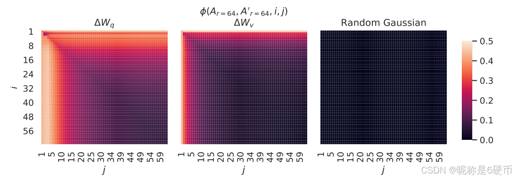
【翻译】图4:左图和中图:第48层中ΔWq\Delta W_{q}ΔWq和ΔWv\Delta W_{v}ΔWv的两个随机种子Ar=64A_{r=64}Ar=64列向量之间的归一化子空间相似性。右图:两个随机高斯矩阵列向量之间的相同热图。其他层见第H.1节。
To answer these questions, we project WWW onto the rrr -dimensional subspace of ΔW\Delta WΔW by computing U⊤WV⊤U^{\top}W V^{\top}U⊤WV⊤ , with U/VU/VU/V being the left/right singular-vector matrix of ΔW\Delta WΔW . Then, we compare the Frobenius norm between ∥U⊤WV⊤ˉ∥F\|U^{\top}W\bar{V^{\top}}\|_{F}∥U⊤WV⊤ˉ∥F and ∥W∥F\|W\|_{F}∥W∥F . As a comparison, we also compute ∥U⊤WV⊤∥F\|U^{\top}W V^{\top}\|_{F}∥U⊤WV⊤∥F by replacing U,VU,VU,V with the top rrr singular vectors of WWW or a random matrix.
【翻译】为了回答这些问题,我们通过计算U⊤WV⊤U^{\top}W V^{\top}U⊤WV⊤将WWW投影到ΔW\Delta WΔW的rrr维子空间上,其中U/VU/VU/V是ΔW\Delta WΔW的左/右奇异向量矩阵。然后,我们比较∥U⊤WV⊤ˉ∥F\|U^{\top}W\bar{V^{\top}}\|_{F}∥U⊤WV⊤ˉ∥F和∥W∥F\|W\|_{F}∥W∥F之间的Frobenius范数。作为比较,我们还通过将U,VU,VU,V替换为WWW的前rrr个奇异向量或随机矩阵来计算∥U⊤WV⊤∥F\|U^{\top}W V^{\top}\|_{F}∥U⊤WV⊤∥F。
Table 7: The Frobenius norm of U⊤WqV⊤U^{\top}W_{q}V^{\top}U⊤WqV⊤ where UUU and VVV are the left/right top rrr singular vector directions of either (1) ΔWq\Delta W_{q}ΔWq , (2) WqW_{q}Wq , or (3) a random matrix. The weight matrices are taken from the 48th48\mathrm{th}48th layer of GPT-3.
【翻译】表7:U⊤WqV⊤U^{\top}W_{q}V^{\top}U⊤WqV⊤的Frobenius范数,其中UUU和VVV是以下三者之一的左/右前rrr个奇异向量方向:(1) ΔWq\Delta W_{q}ΔWq,(2) WqW_{q}Wq,或(3) 随机矩阵。权重矩阵取自GPT-3的第48层。
We draw several conclusions from Table 7. First, ΔW\Delta WΔW has a stronger correlation with WWW compared to a random matrix, indicating that ΔW\Delta WΔW amplifies some features that are already in WWW . Second, instead of repeating the top singular directions of WWW , ΔW\Delta WΔW only amplifies directions that are not emphasized in WWW . Third, the amplification factor is rather huge: 21.5≈6.91/0.3221.5\approx6.91/0.3221.5≈6.91/0.32 for r=4r=4r=4 . See Section H.4 for why r=64r=64r=64 has a smaller amplification factor. We also provide a visualization in Section H.3 for how the correlation changes as we include more top singular directions from WqW_{q}Wq . This suggests that the low-rank adaptation matrix potentially amplifies the important features for specific downstream tasks that were learned but not emphasized in the general pre-training model.
【翻译】我们从表7中得出几个结论。首先,与随机矩阵相比,ΔW\Delta WΔW与WWW有更强的相关性,表明ΔW\Delta WΔW放大了WWW中已经存在的一些特征。其次,ΔW\Delta WΔW不是重复WWW的顶部奇异方向,而是只放大WWW中未被强调的方向。第三,放大因子相当巨大:对于r=4r=4r=4,21.5≈6.91/0.3221.5\approx6.91/0.3221.5≈6.91/0.32。参见第H.4节了解为什么r=64r=64r=64有较小的放大因子。我们还在第H.3节中提供了一个可视化,展示当我们包含更多来自WqW_{q}Wq的顶部奇异方向时相关性如何变化。这表明低秩适应矩阵可能放大了在通用预训练模型中学到但未被强调的特定下游任务的重要特征。
8 结论与未来工作
Fine-tuning enormous language models is prohibitively expensive in terms of the hardware required and the storage/switching cost for hosting independent instances for different tasks. We propose LoRA, an efficient adaptation strategy that neither introduces inference latency nor reduces input sequence length while retaining high model quality. Importantly, it allows for quick task-switching when deployed as a service by sharing the vast majority of the model parameters. While we focused on Transformer language models, the proposed principles are generally applicable to any neural networks with dense layers.
【翻译】微调庞大的语言模型在所需硬件以及为不同任务托管独立实例的存储/切换成本方面是极其昂贵的。我们提出LoRA,一种高效的适应策略,既不引入推理延迟,也不减少输入序列长度,同时保持高模型质量。重要的是,当作为服务部署时,它通过共享绝大多数模型参数来实现快速任务切换。虽然我们专注于Transformer语言模型,但所提出的原理通常适用于任何具有密集层的神经网络。
There are many directions for future works. 1) LoRA can be combined with other efficient adaptation methods, potentially providing orthogonal improvement. 2) The mechanism behind fine-tuning or LoRA is far from clear – how are features learned during pre-training transformed to do well on downstream tasks? We believe that LoRA makes it more tractable to answer this than full finetuning. 3) We mostly depend on heuristics to select the weight matrices to apply LoRA to. Are there more principled ways to do it? 4) Finally, the rank-deficiency of ΔW\Delta WΔW suggests that WWW could be rank-deficient as well, which can also be a source of inspiration for future works.
【翻译】未来工作有许多方向。1) LoRA可以与其他高效适应方法结合,可能提供正交改进。2) 微调或LoRA背后的机制远未清楚——预训练期间学习的特征是如何转换为在下游任务中表现良好的?我们相信LoRA比完全微调更容易回答这个问题。3) 我们主要依靠启发式方法来选择应用LoRA的权重矩阵。是否有更有原则的方法来做到这一点?4) 最后,ΔW\Delta WΔW的秩不足表明WWW也可能是秩不足的,这也可以成为未来工作的灵感来源。