Python5-线性回归
提示:文章写完后,目录可以自动生成,如何生成可参考右边的帮助文档
文章目录
- 前言
- 1. 线性回归简介
- 2. 线性回归api初步使⽤
- 3. 数学:求导
- 3.1 矩阵(向量)求导[了解]
- 4. 线性回归的损失和优化
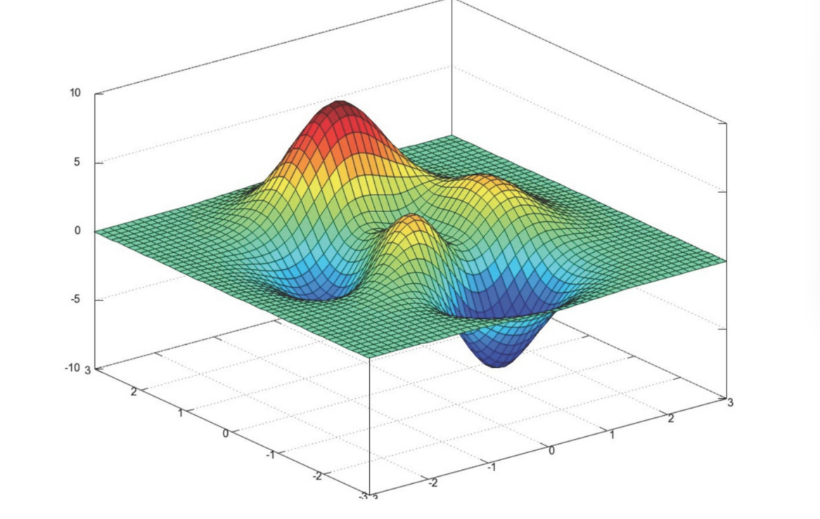
- 4.1 正规⽅程
- 4.2 正规⽅程的推导
- 4.3 梯度下降(Gradient Descent)
- 5. 梯度下降⽅法介绍
- 6. 线性回归api再介绍
- 7. 案例:波⼠顿房价预测
- 7.1 正规⽅程
- 7.2 梯度下降法
- 8. ⽋拟合和过拟合
- 8.1 正则化
- 9. 正则化线性模型
- 9.1 Ridge Regression (岭回归,⼜名 Tikhonov regularization)
- 9.2 Lasso Regression(Lasso 回归)
- 9.3 Elastic Net (弹性⽹络)
- 10. 线性回归的改进-岭回归
- 10.1 API
- 11. 模型的保存和加载
- 11.1 sklearn模型的保存和加载API
- 总结
前言
1. 线性回归简介
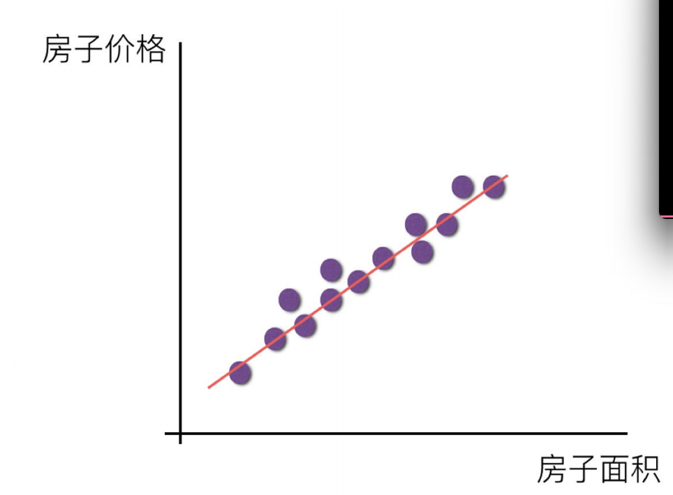
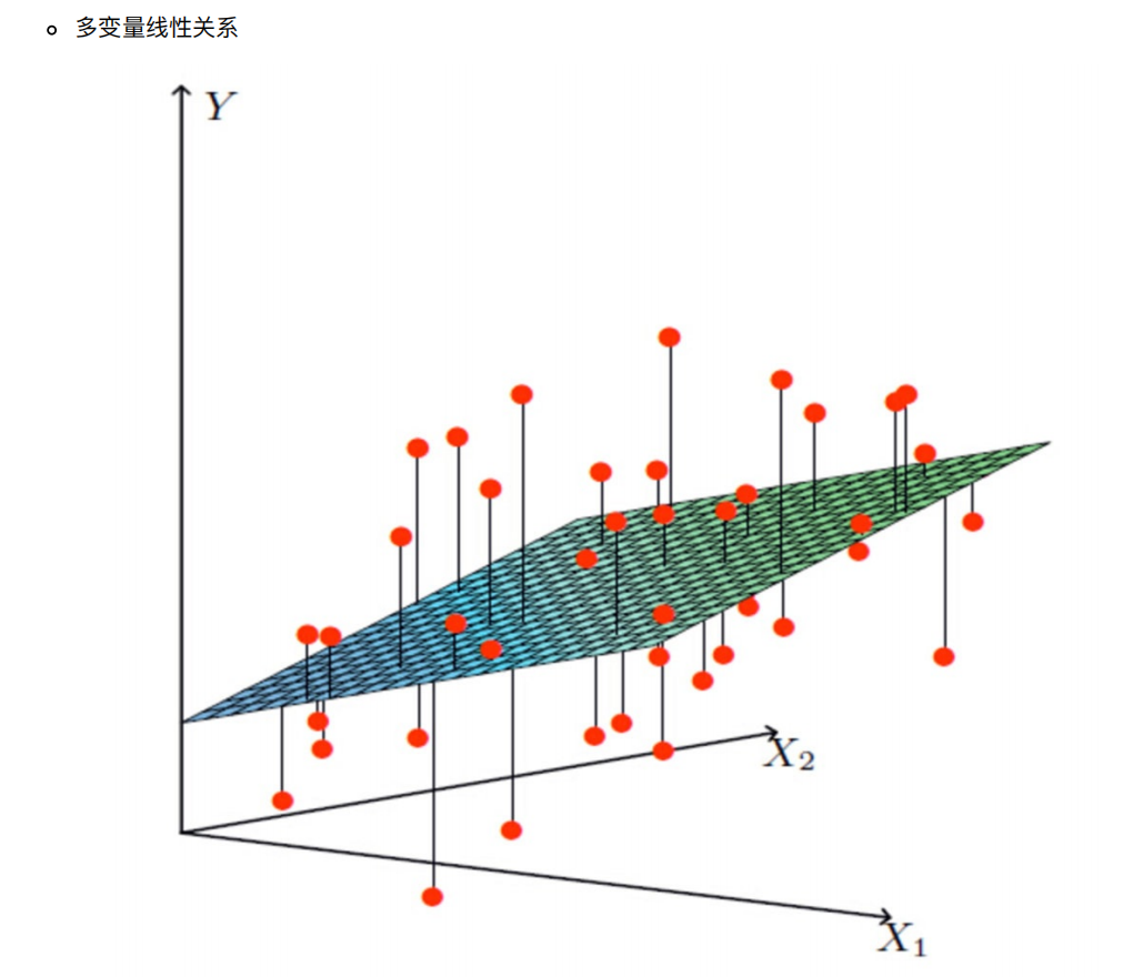
线性回归(Linear regression)是利⽤回归⽅程(函数)对⼀个或多个⾃变量(特征值)和因变量(⽬标值)之间关系进⾏建模的
⼀种分析⽅式。
特点:只有⼀个⾃变量的情况称为单变量回归,多于⼀个⾃变量情况的叫做多元回归
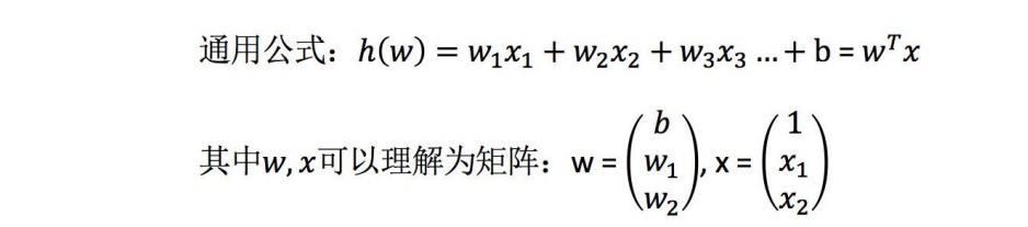
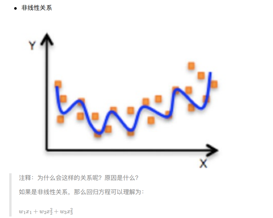
线性回归当中主要有两种模型,⼀种是线性关系,另⼀种是⾮线性关系
2. 线性回归api初步使⽤
sklearn.linear_model.LinearRegression()
LinearRegression.coef_:回归系数
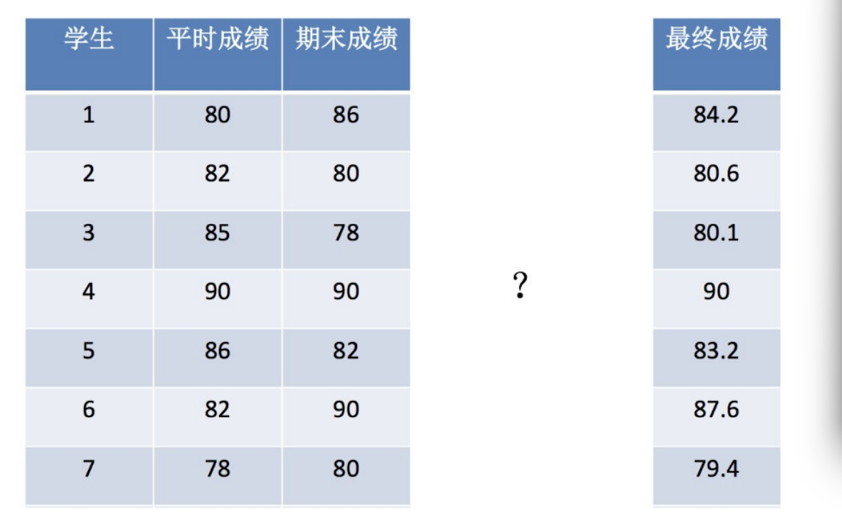
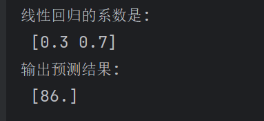
from sklearn.linear_model import LinearRegressionx = [[80, 86],[82, 80],[85, 78],[90, 90],[86, 82],[82, 90],[78, 80],[92, 94]]
y = [84.2, 80.6, 80.1, 90, 83.2, 87.6, 79.4, 93.4]
#实例化一个估计器
estimator = LinearRegression()
#fit进行训练
estimator.fit(x,y)
#打印对应的系数
print("线性回归的系数是:\n",estimator.coef_)
print("输出预测结果:\n",estimator.predict([[100,80]]))
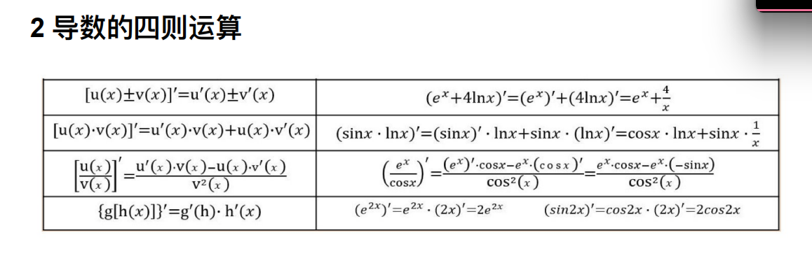
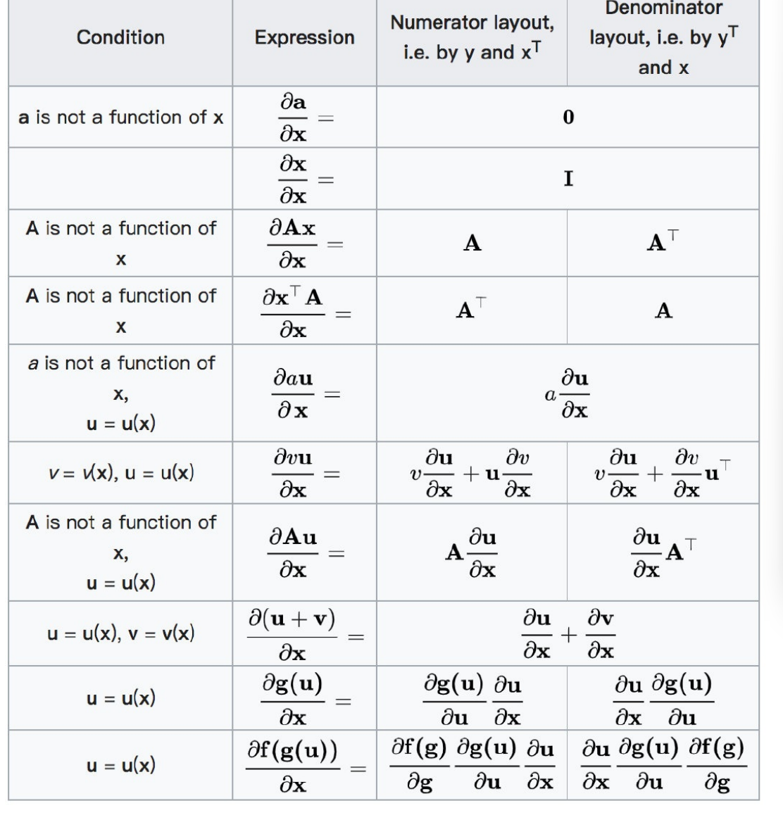
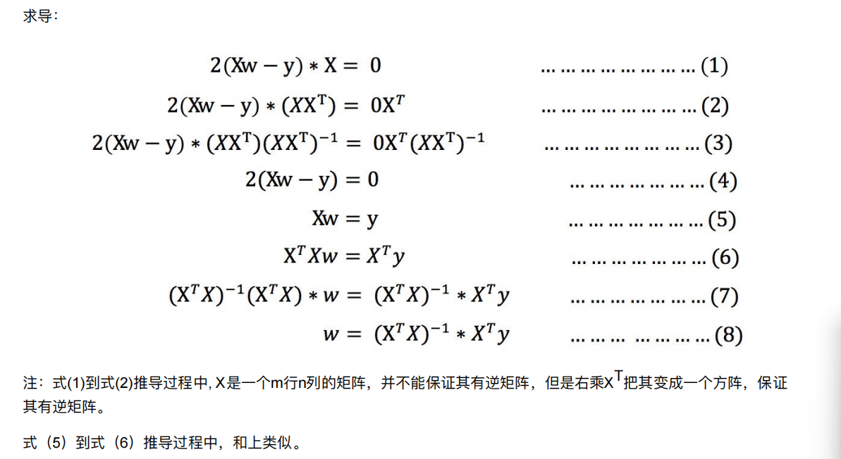
3. 数学:求导
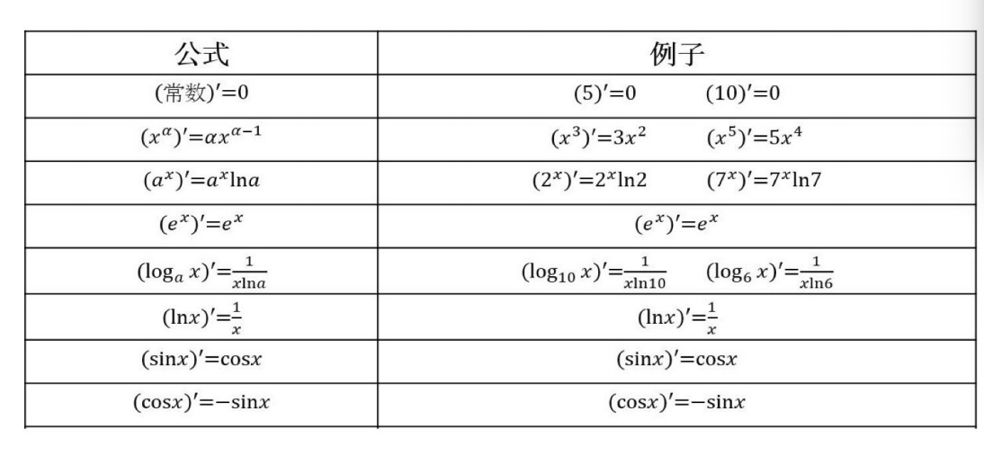
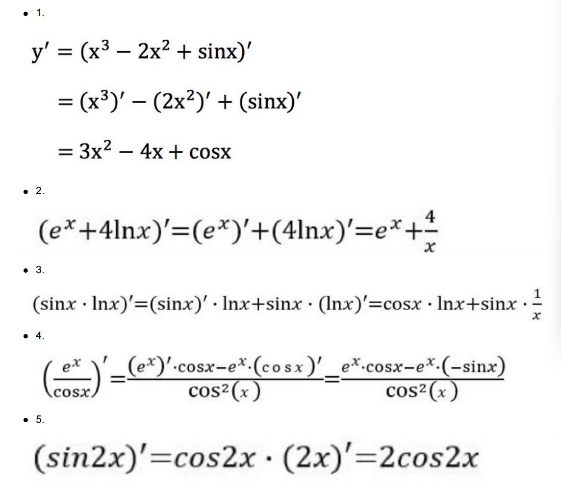
3.1 矩阵(向量)求导[了解]
4. 线性回归的损失和优化
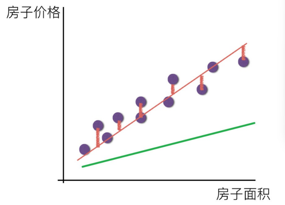
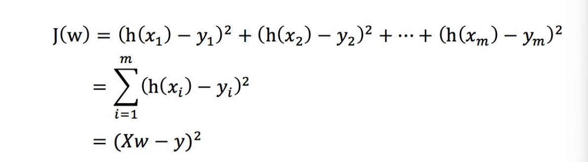
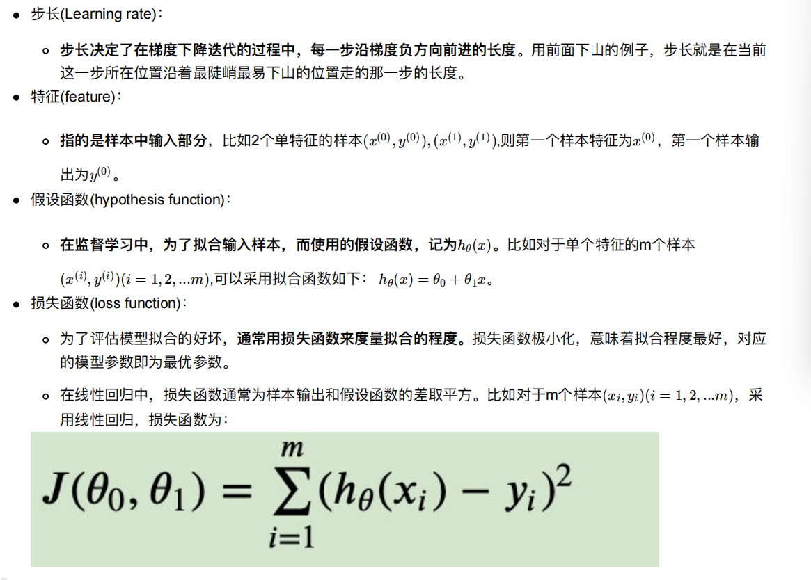
既然存在这个误差,那我们就将这个误差给衡量出来
损失函数
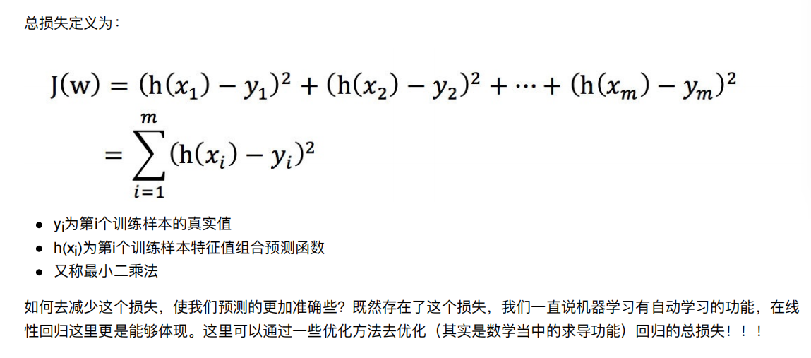
如何去求模型当中的W,使得损失最⼩?(⽬的是找到最⼩损失对应的W值)
线性回归经常使⽤的两种优化算法
正规⽅程
梯度下降法
4.1 正规⽅程
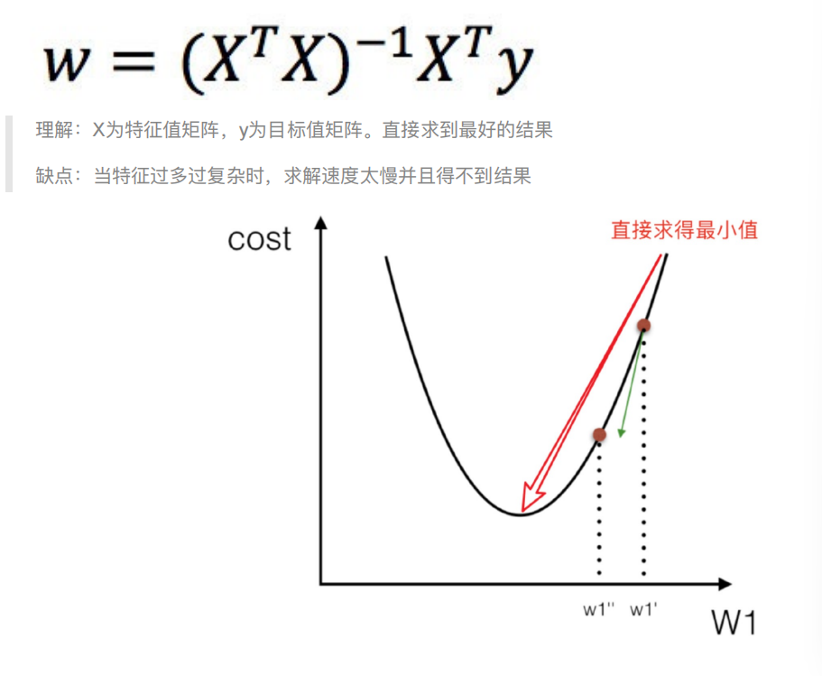
–》很难求解
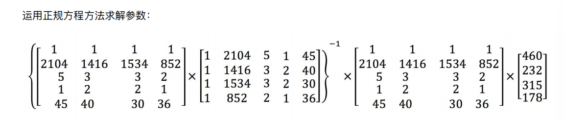
4.2 正规⽅程的推导
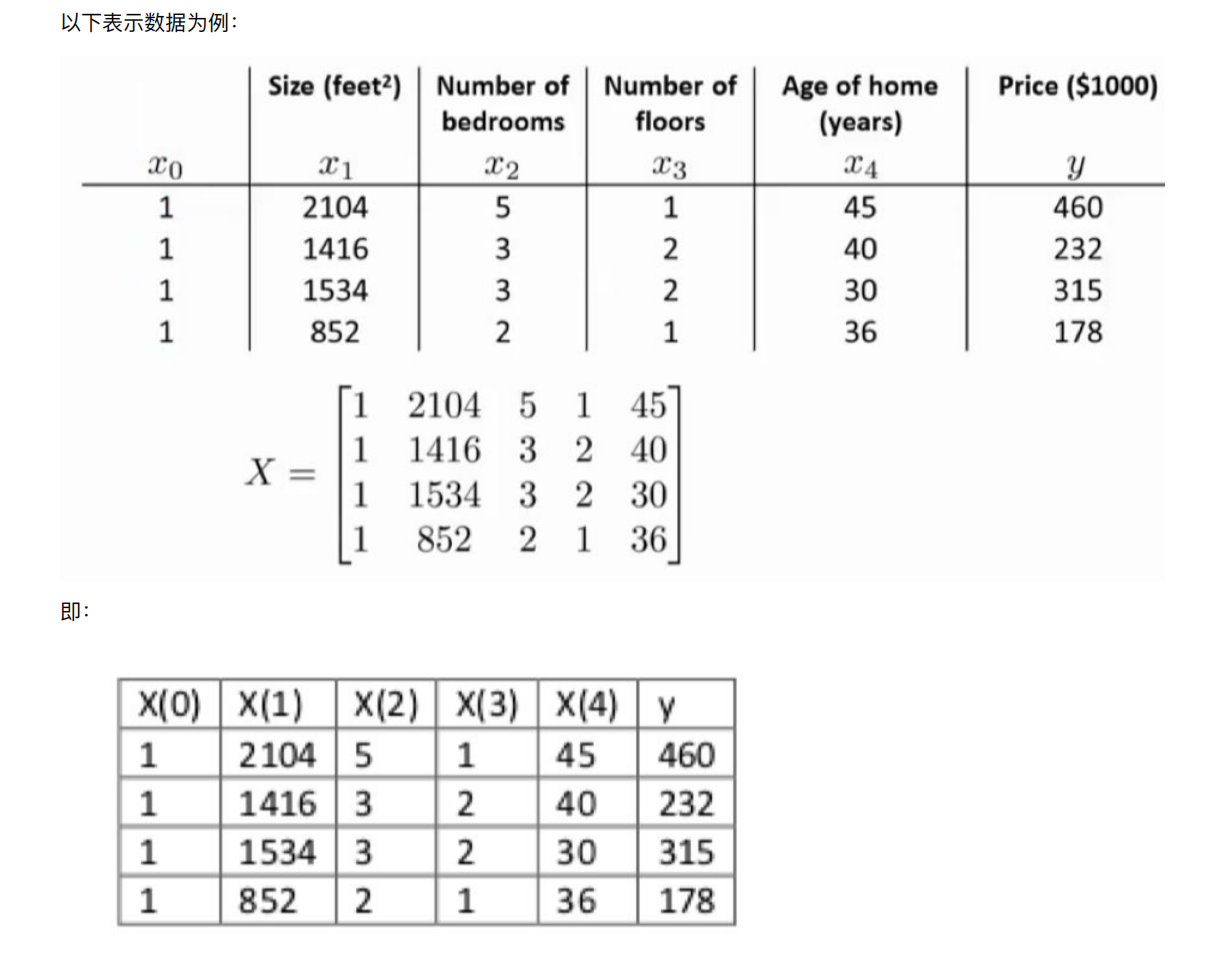
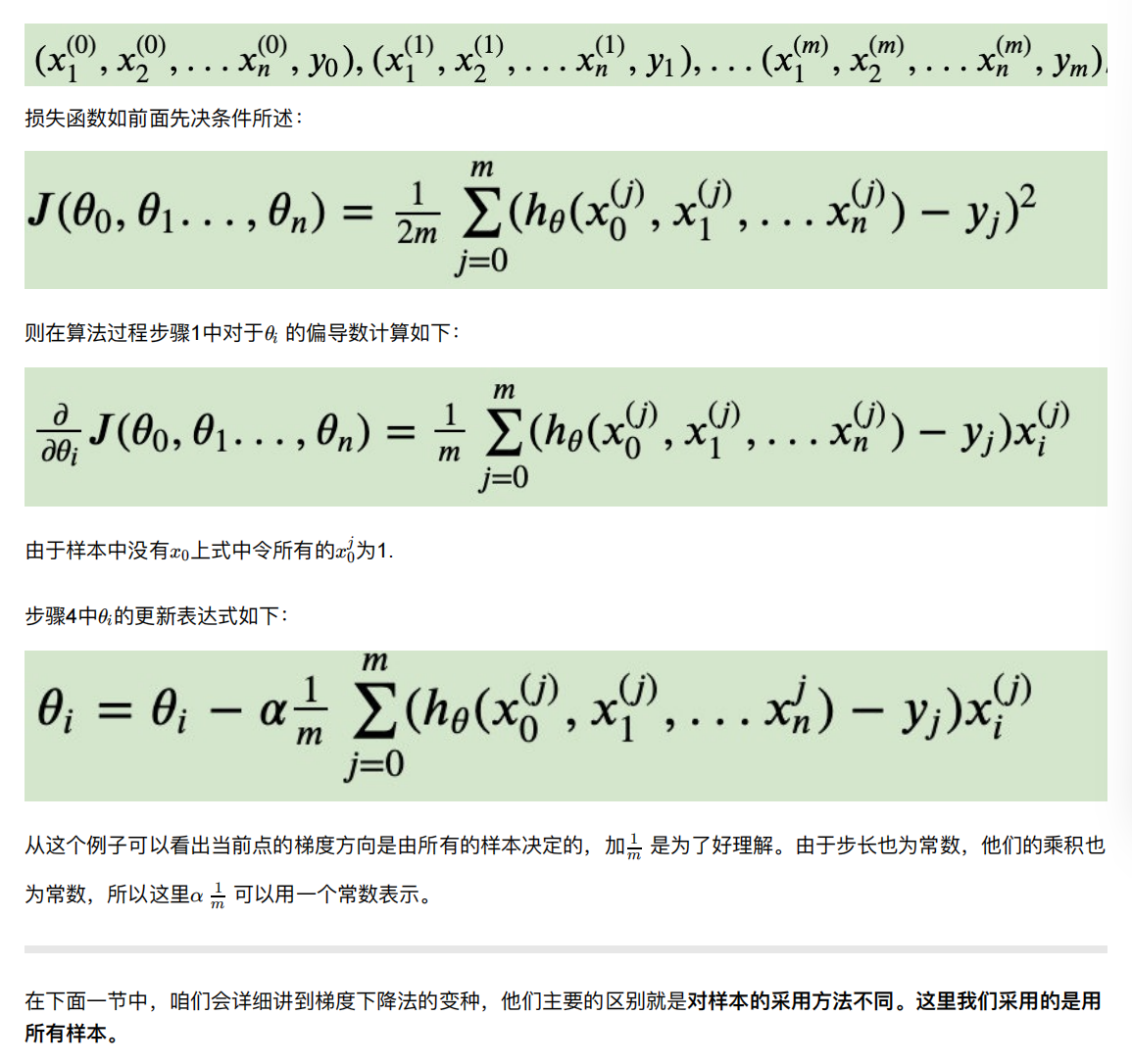
其中y是真实值矩阵,X是特征值矩阵,w是权重矩阵
对其求解关于w的最⼩值,起⽌y,X 均已知⼆次函数直接求导,导数为零的位置,即为最⼩值。
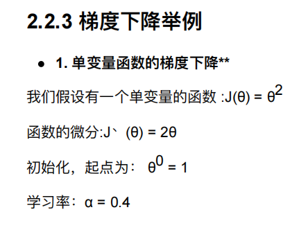
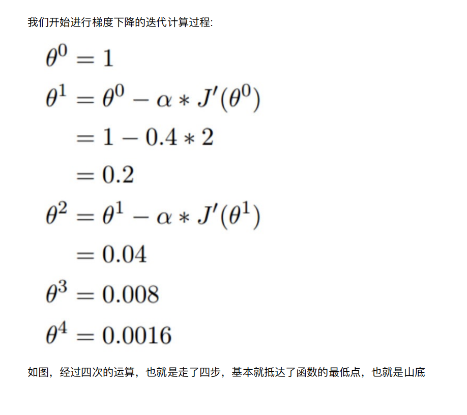
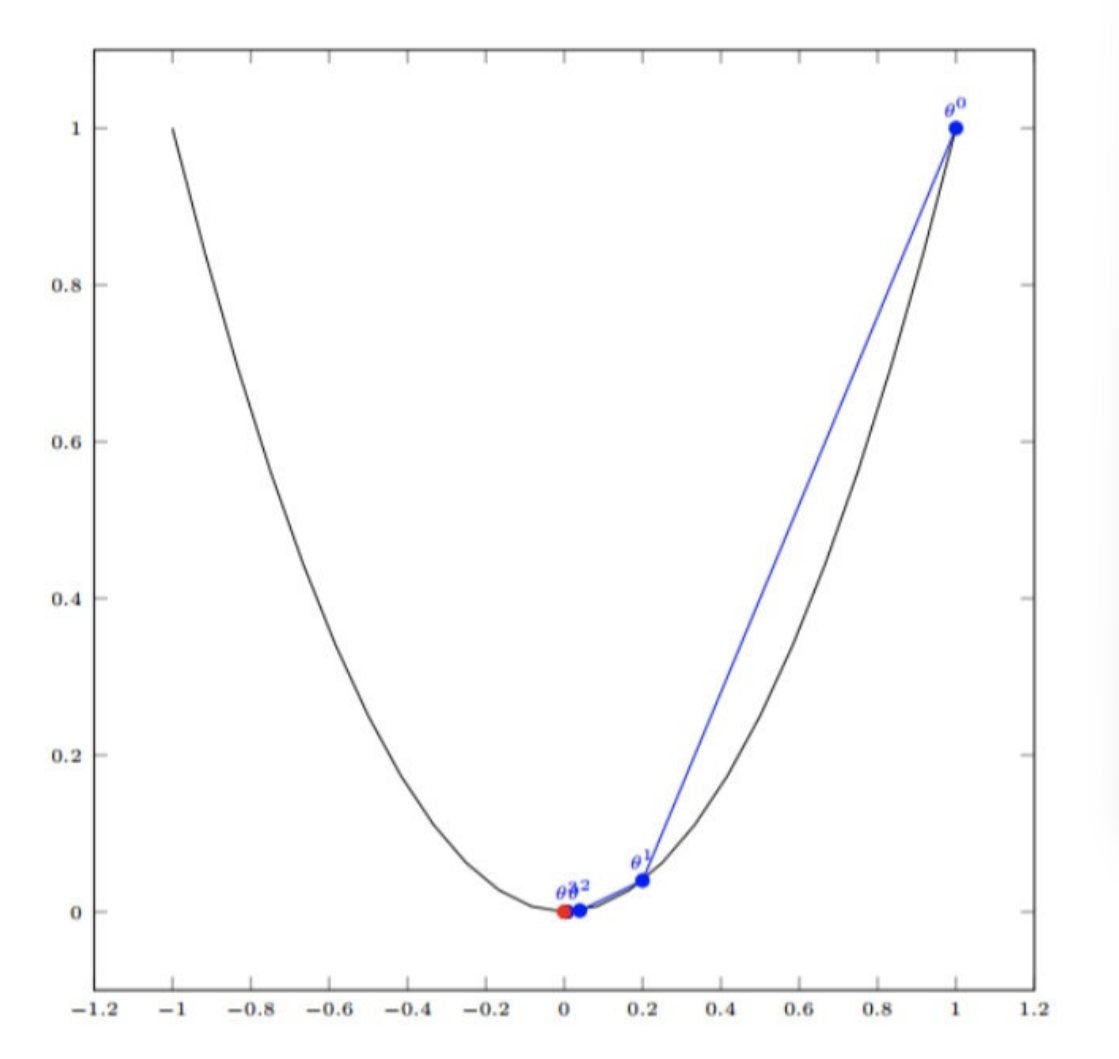
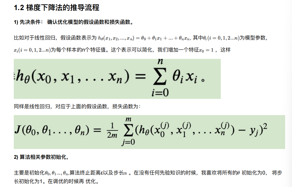
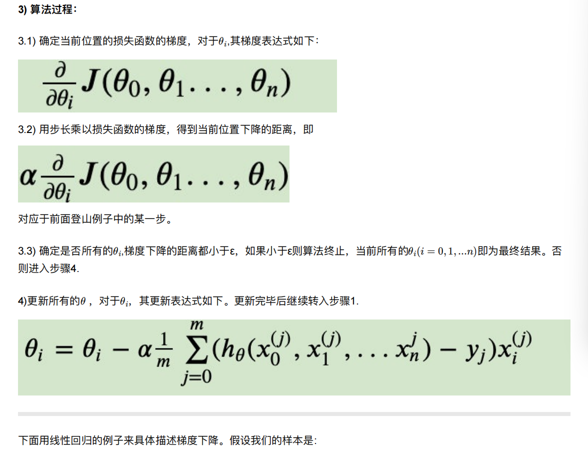
4.3 梯度下降(Gradient Descent)
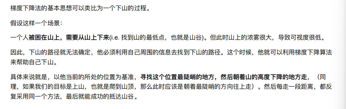
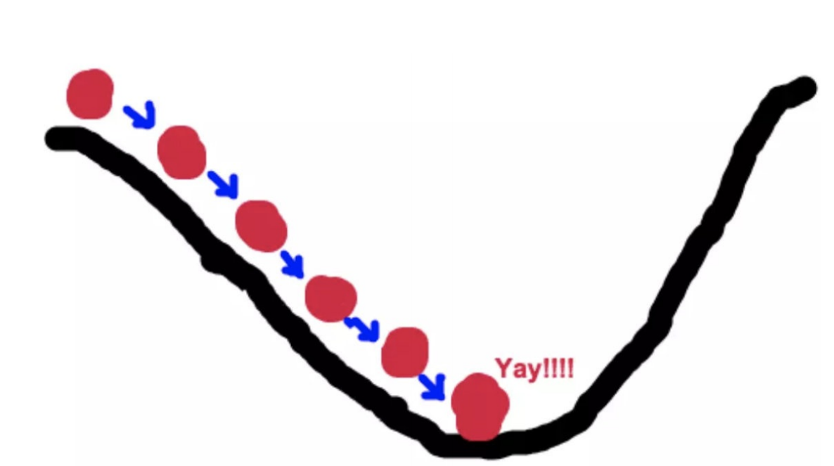
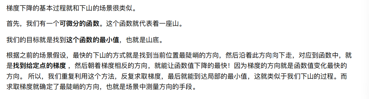
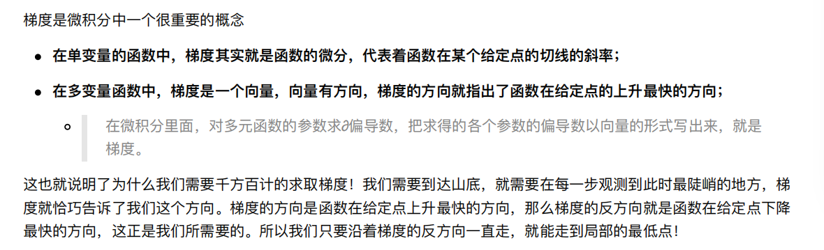
就是横坐标一直减去axk
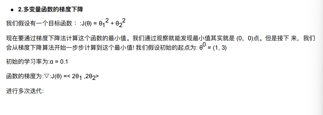
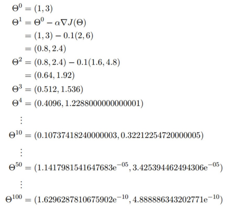
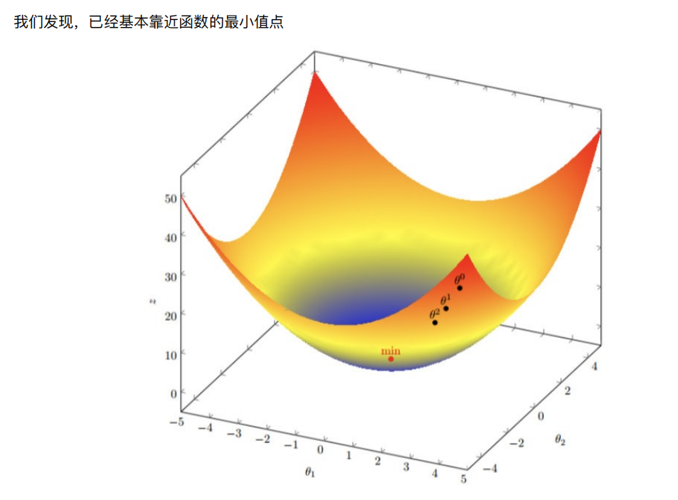
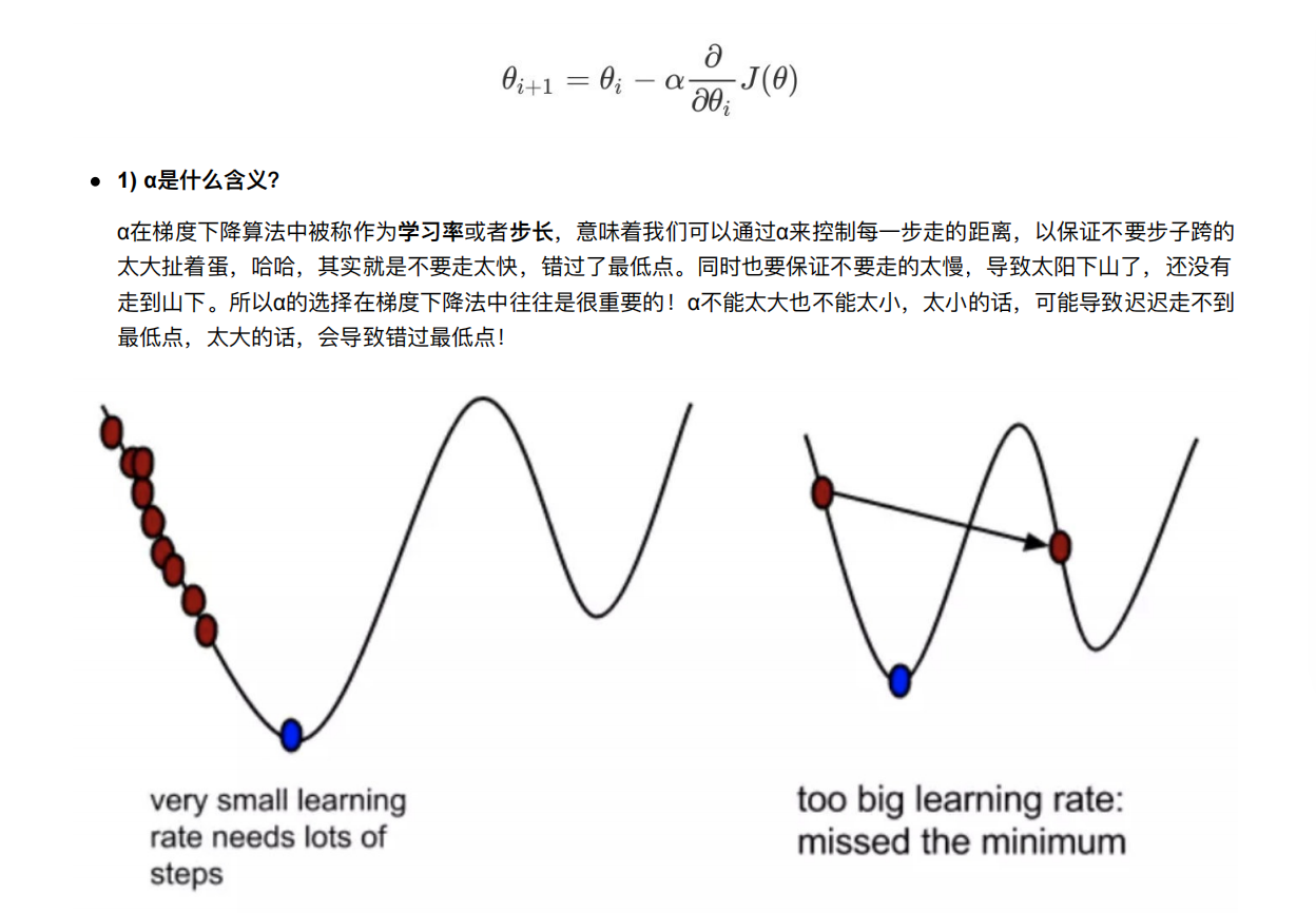
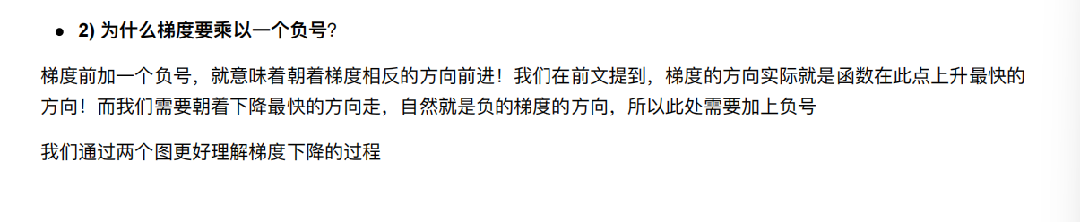
只能保证走到了极小值,不能是最小值
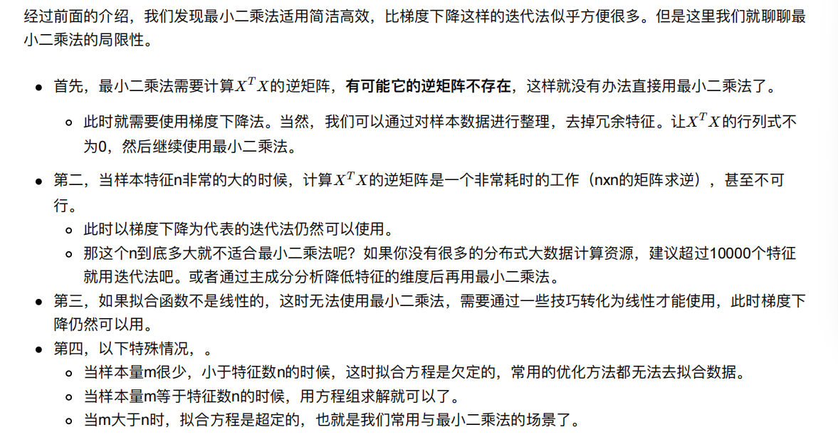
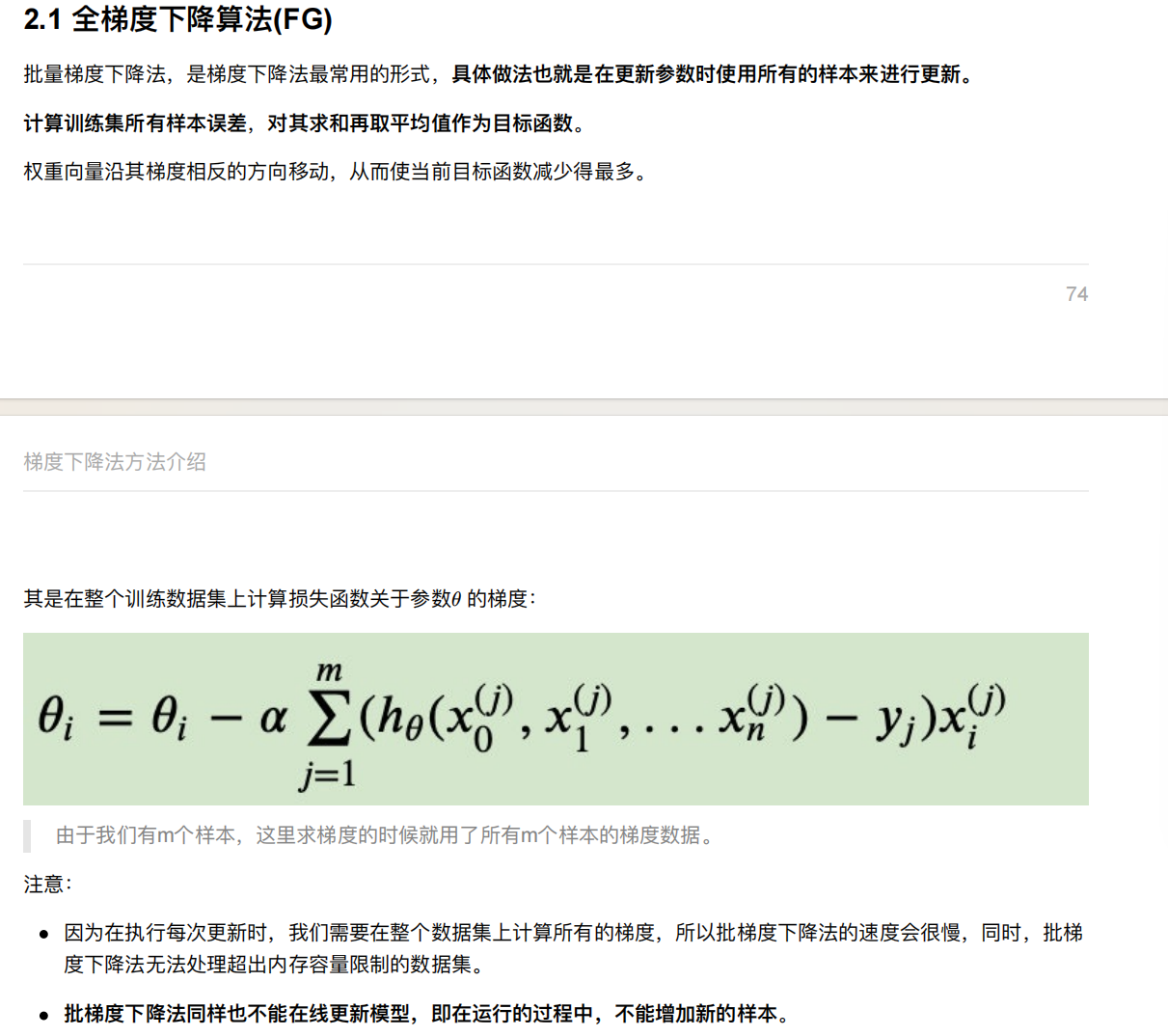
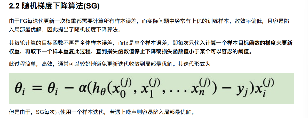
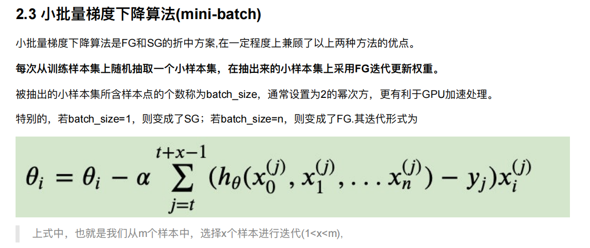
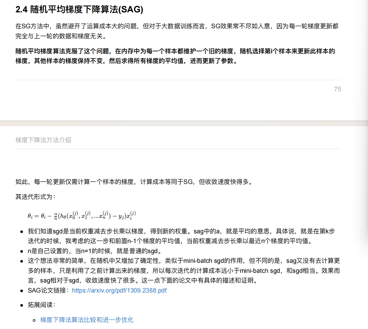
5. 梯度下降⽅法介绍
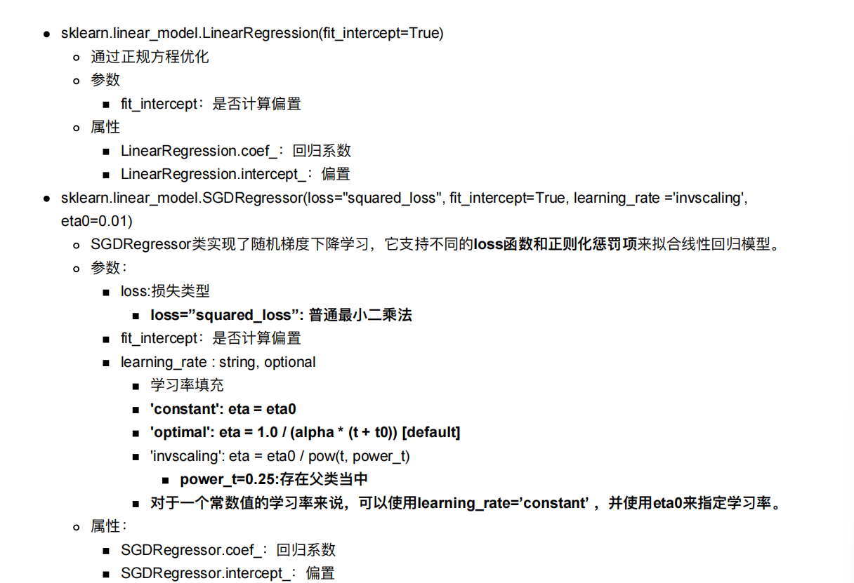
6. 线性回归api再介绍
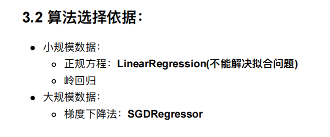
sklearn.linear_model.LinearRegression(fit_intercept=True)通过正规⽅程优化参数fit_intercept:是否计算偏置属性LinearRegression.coef_:回归系数LinearRegression.intercept_:偏置
sklearn.linear_model.SGDRegressor(loss="squared_loss", fit_intercept=True, learning_rate ='invscaling',
eta0=0.01)SGDRegressor类实现了随机梯度下降学习,它⽀持不同的loss函数和正则化惩罚项来拟合线性回归模型。参数:loss:损失类型loss=”squared_loss”: 普通最⼩⼆乘法fit_intercept:是否计算偏置learning_rate : string, optional学习率填充'constant': eta = eta0'optimal': eta = 1.0 / (alpha * (t + t0)) [default]'invscaling': eta = eta0 / pow(t, power_t)power_t=0.25:存在⽗类当中对于⼀个常数值的学习率来说,可以使⽤learning_rate=’constant’ ,并使⽤eta0来指定学习率。属性:SGDRegressor.coef_:回归系数SGDRegressor.intercept_:偏置
y=ax+b
回归系数就是a,偏置就是b
SGDRegressor是随机梯度下降的方法
LinearRegression是正规方程的方法
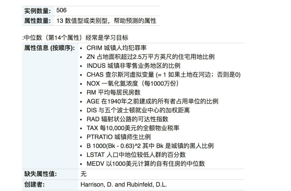
7. 案例:波⼠顿房价预测
7.1 正规⽅程
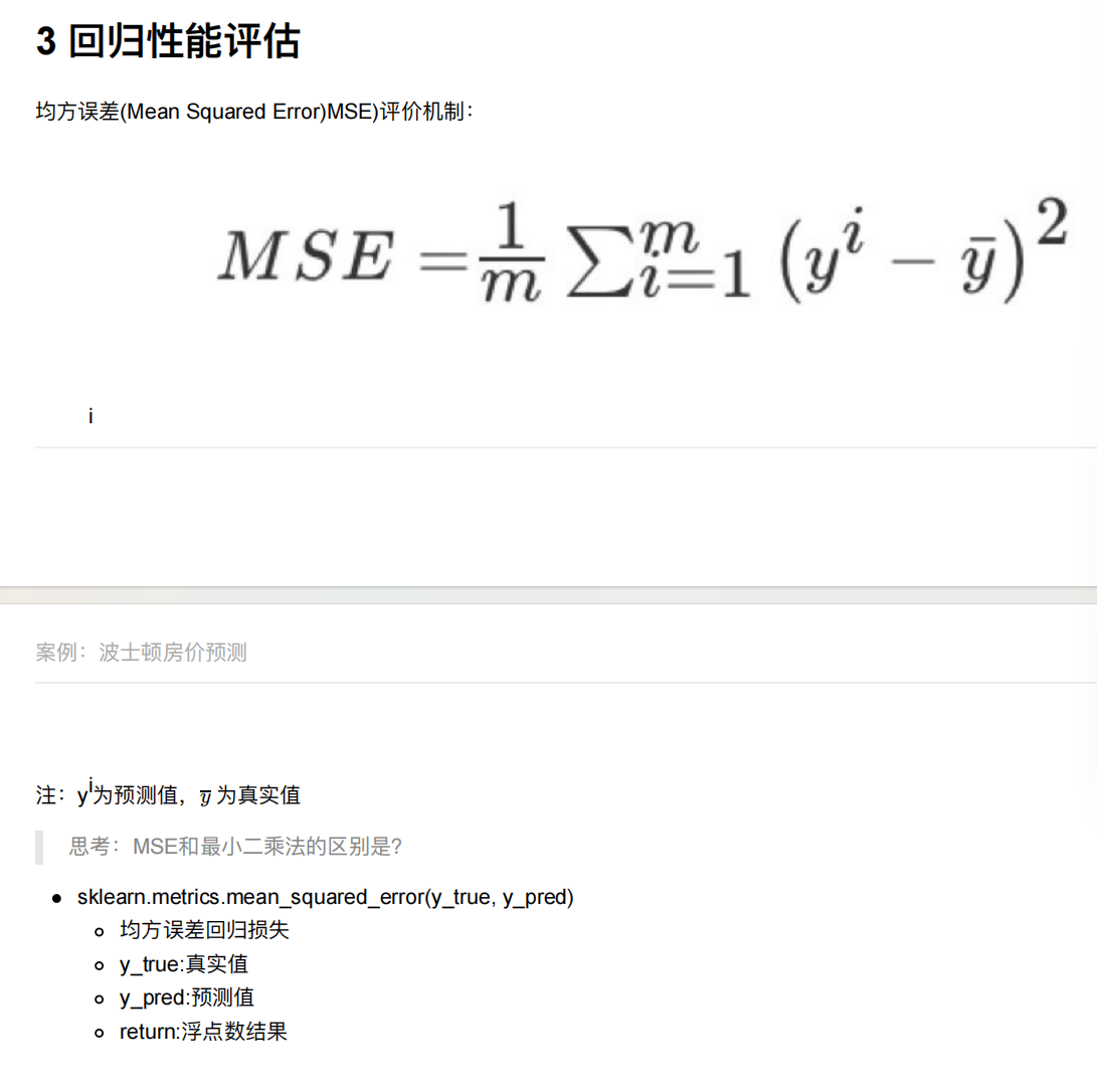
sklearn.metrics.mean_squared_error(y_true, y_pred)
均⽅误差回归损失
y_true:真实值
y_pred:预测值
return:浮点数结果
返回的就是均方误差
#1. 获取数据 加州房价数据集
from sklearn.datasets import fetch_california_housing
#2.分割数据
from sklearn.model_selection import train_test_split
#3. 特征工程--标准化
from sklearn.preprocessing import StandardScaler
#4. 机器学习-线性回归
from sklearn.linear_model import LinearRegression
#5. 模型评估
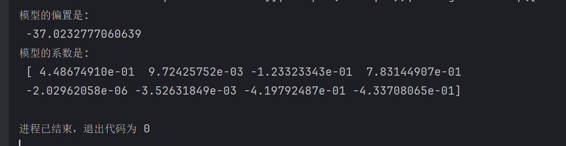
from sklearn.metrics import mean_squared_errordef linear_model():# 1. 获取数据housing = fetch_california_housing()print(housing)# 2.数据基本处理# 2.1 分割数据x_train, x_test, y_train, y_test = train_test_split(housing.data, housing.target,test_size=0.2,random_state=42)# 3. 特征工程--标准化transfer = StandardScaler()transfer.fit_transform(x_train)transfer.transform(x_test)# 4. 机器学习-线性回归estimator = LinearRegression()estimator.fit(x_train, y_train)print("模型的偏置是:\n",estimator.intercept_)print("模型的系数是:\n",estimator.coef_)# 5. 模型评估linear_model()
#正规方程
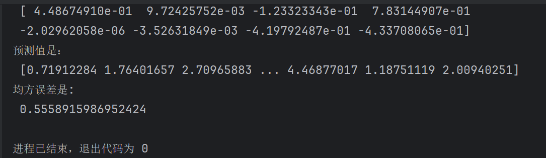
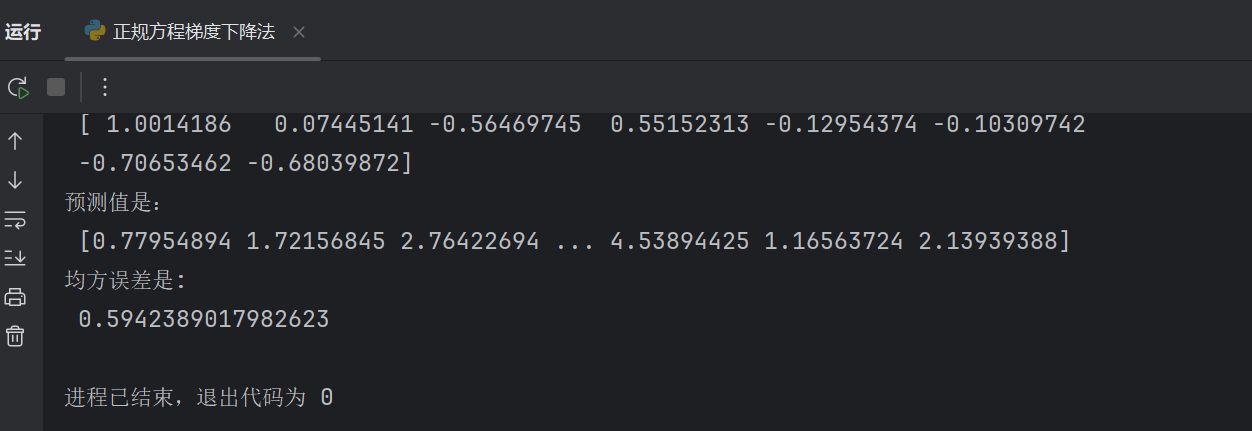
def linear_model1():# 1. 获取数据housing = fetch_california_housing()print(housing)# 2.数据基本处理# 2.1 分割数据x_train, x_test, y_train, y_test = train_test_split(housing.data, housing.target,test_size=0.2,random_state=42)# 3. 特征工程--标准化transfer = StandardScaler()x_train=transfer.fit_transform(x_train)x_test=transfer.transform(x_test)# 4. 机器学习-线性回归estimator = LinearRegression()estimator.fit(x_train, y_train)print("模型的偏置是:\n",estimator.intercept_)print("模型的系数是:\n",estimator.coef_)# 5. 模型评估#5.1 预测值y_pre=estimator.predict(x_test)print("预测值是:\n",y_pre)#5.2 均方误差mse = mean_squared_error(y_test,y_pre)print("均方误差是:\n",mse)
7.2 梯度下降法
#1. 获取数据  加州房价数据集
from sklearn.datasets import fetch_california_housing
#2.分割数据
from sklearn.model_selection import train_test_split
#3. 特征工程--标准化
from sklearn.preprocessing import StandardScaler
#4. 机器学习-线性回归
from sklearn.linear_model import LinearRegression,SGDRegressor
#5. 模型评估
from sklearn.metrics import mean_squared_error
#梯度下降法
def linear_model2():# 1. 获取数据housing  = fetch_california_housing()print(housing)# 2.数据基本处理# 2.1 分割数据x_train, x_test, y_train, y_test = train_test_split(housing.data, housing.target,test_size=0.2,random_state=42)# 3. 特征工程--标准化transfer = StandardScaler()x_train=transfer.fit_transform(x_train)x_test=transfer.transform(x_test)# 4. 机器学习-线性回归# estimator = SGDRegressor(max_iter=1000)estimator = SGDRegressor(max_iter=1000)estimator.fit(x_train, y_train)print("模型的偏置是:\n",estimator.intercept_)print("模型的系数是:\n",estimator.coef_)# 5. 模型评估#5.1 预测值y_pre=estimator.predict(x_test)print("预测值是:\n",y_pre)#5.2 均方误差mse = mean_squared_error(y_test,y_pre)print("均方误差是:\n",mse)
max_iter=1000 表示最大迭代次数
estimator = SGDRegressor(max_iter=1000,learning_rate="constant",eta0=1)
learning_rate="constant"表示学习率的更新策略为 “恒定不变”。
其他常见策略还有:“optimal”(自适应调整)、“invscaling”(随迭代次数衰减)等。
eta0=1表示初始学习率的大小,仅在 learning_rate 为 “constant” 或 “invscaling” 时生效。此处设置为 1,意味着模型在训练开始时,每次参数更新的步长为 1(后续若策略为恒定,则保持 1 不变)。
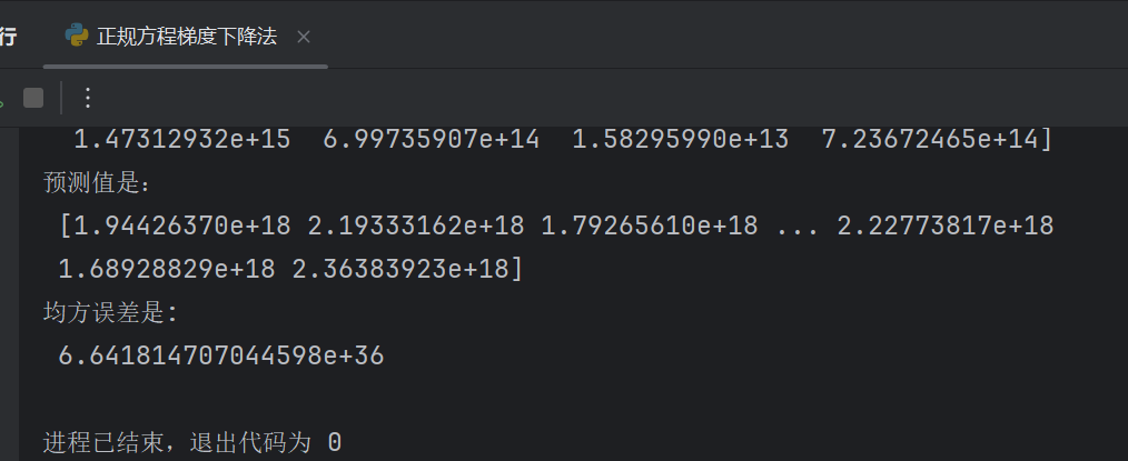
发现误差都变大了,是以e为单位的
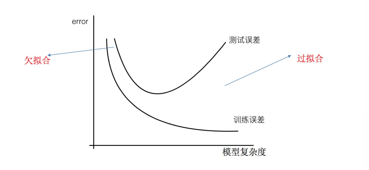
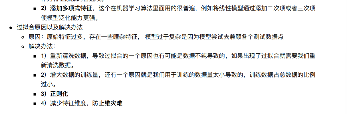
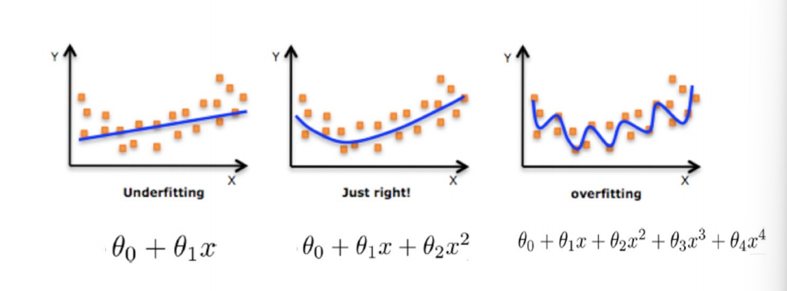
8. ⽋拟合和过拟合
过拟合:⼀个假设在训练数据上能够获得⽐其他假设更好的拟合, 但是在测试数据集上却不能很好地拟合数据,
此时认为这个假设出现了过拟合的现象。(模型过于复杂)
⽋拟合:⼀个假设在训练数据上不能获得更好的拟合,并且在测试数据集上也不能很好地拟合数据,此时认为这个
假设出现了⽋拟合的现象。(模型过于简单)
8.1 正则化
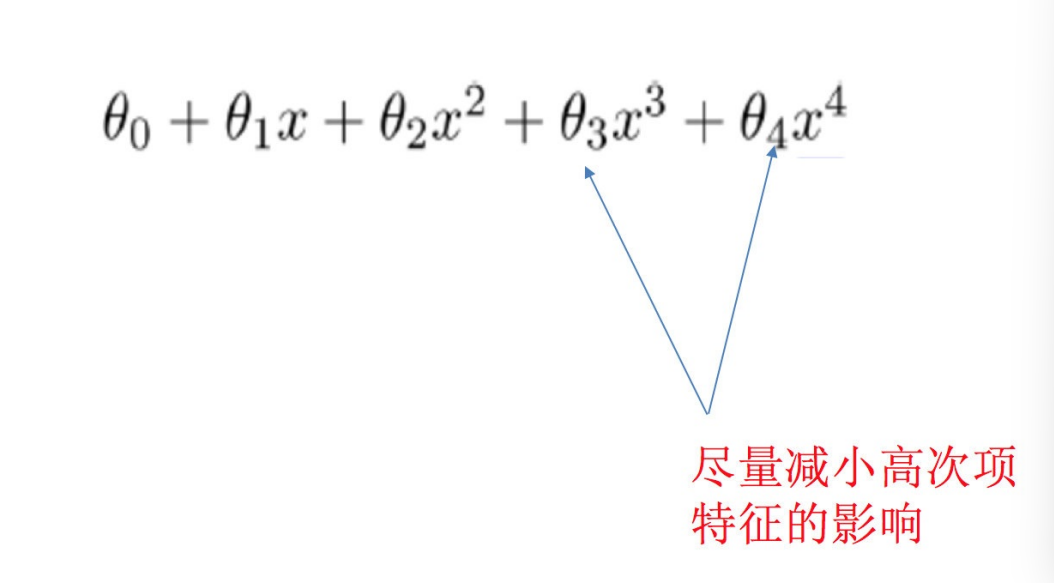
在学习的时候,数据提供的特征有些影响模型复杂度或者这个特征的数据点异常较多,所以算法在学习的时候尽量减少
这个特征的影响(甚⾄删除某个特征的影响),这就是正则化
注:调整时候,算法并不知道某个特征影响,⽽是去调整参数得出优化的结果
正则化类别
L2正则化
作⽤:可以使得其中⼀些W的都很⼩,都接近于0,削弱某个特征的影响
优点:越⼩的参数说明模型越简单,越简单的模型则越不容易产⽣过拟合现象
Ridge回归
L1正则化
作⽤:可以使得其中⼀些W的值直接为0,删除这个特征的影响
LASSO回归
9. 正则化线性模型
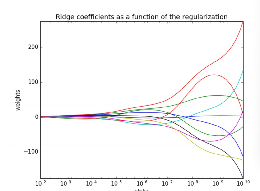
9.1 Ridge Regression (岭回归,⼜名 Tikhonov regularization)
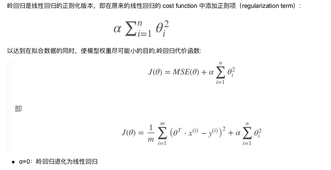
当平方太大了,a就变小,平方太小了,a就变大,a就是一个惩罚力度
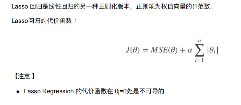
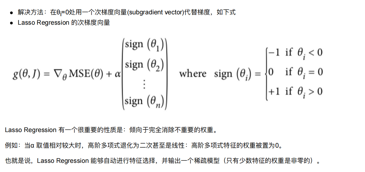
9.2 Lasso Regression(Lasso 回归)
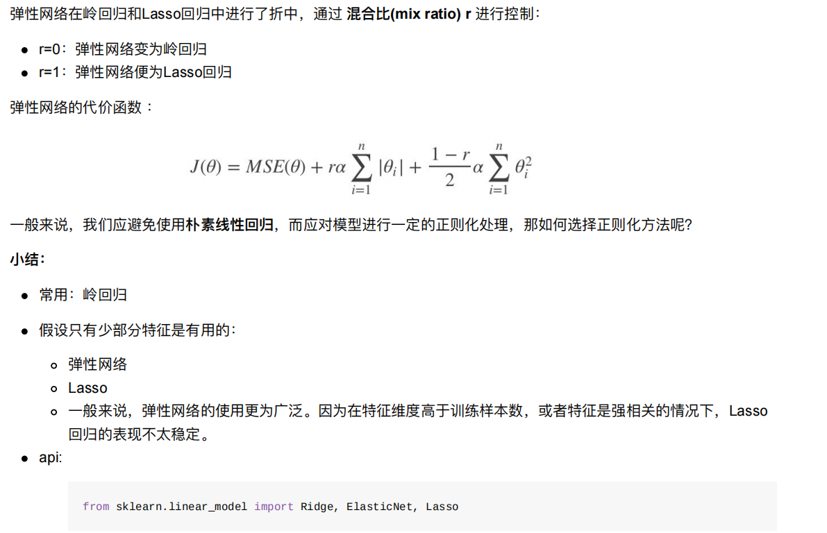
9.3 Elastic Net (弹性⽹络)
10. 线性回归的改进-岭回归
10.1 API
sklearn.linear_model.Ridge(alpha=1.0, fit_intercept=True,solver="auto", normalize=False)具有l2正则化的线性回归alpha:正则化⼒度,也叫 λλ取值:0~1 1~10solver:会根据数据⾃动选择优化⽅法sag:如果数据集、特征都⽐较⼤,选择该随机梯度下降优化normalize:数据是否进⾏标准化normalize=False:可以在fit之前调⽤preprocessing.StandardScaler标准化数据Ridge.coef_:回归权重Ridge.intercept_:回归偏置
Ridge⽅法相当于SGDRegressor(penalty=‘l2’, loss=“squared_loss”),只不过SGDRegressor实现了⼀个普通的随机
梯度下降学习,推荐使⽤Ridge(实现了SAG)
sklearn.linear_model.RidgeCV(_BaseRidgeCV, RegressorMixin)具有l2正则化的线性回归,可以进⾏交叉验证coef_:回归系数
正则化⼒度越⼤,权重系数会越⼩
正则化⼒度越⼩,权重系数会越⼤
#1. 获取数据  加州房价数据集
from sklearn.datasets import fetch_california_housing
#2.分割数据
from sklearn.model_selection import train_test_split
#3. 特征工程--标准化
from sklearn.preprocessing import StandardScaler
#4. 机器学习-线性回归
from sklearn.linear_model import LinearRegression,SGDRegressor,Ridge,RidgeCV
#5. 模型评估
from sklearn.metrics import mean_squared_error
#岭回归
def linear_model3():# 1. 获取数据housing  = fetch_california_housing()print(housing)# 2.数据基本处理# 2.1 分割数据x_train, x_test, y_train, y_test = train_test_split(housing.data, housing.target,test_size=0.2,random_state=42)# 3. 特征工程--标准化transfer = StandardScaler()x_train=transfer.fit_transform(x_train)x_test=transfer.transform(x_test)# 4. 机器学习-线性回归estimator = Ridge(alpha=1)estimator.fit(x_train, y_train)print("模型的偏置是:\n",estimator.intercept_)print("模型的系数是:\n",estimator.coef_)# 5. 模型评估#5.1 预测值y_pre=estimator.predict(x_test)print("预测值是:\n",y_pre)#5.2 均方误差mse = mean_squared_error(y_test,y_pre)print("均方误差是:\n",mse)
在 Ridge(alpha=1) 中,alpha 是 正则化强度参数,用于控制 Ridge 回归(岭回归)中的 L2 正则化力度,具体含义如下:
作用:L2 正则化会在损失函数中加入一个惩罚项(模型系数的平方和乘以 alpha),限制模型系数的绝对值过大,从而防止过拟合。
取值含义:
alpha 值越大,正则化强度越强,对系数的惩罚越严厉,系数会被压缩得更接近 0,模型复杂度降低(可能欠拟合)。
alpha 值越小,正则化强度越弱,模型更接近普通线性回归(当 alpha=0 时,退化为普通线性回归,但实际使用中不建议这么做,可能导致数值不稳定)。
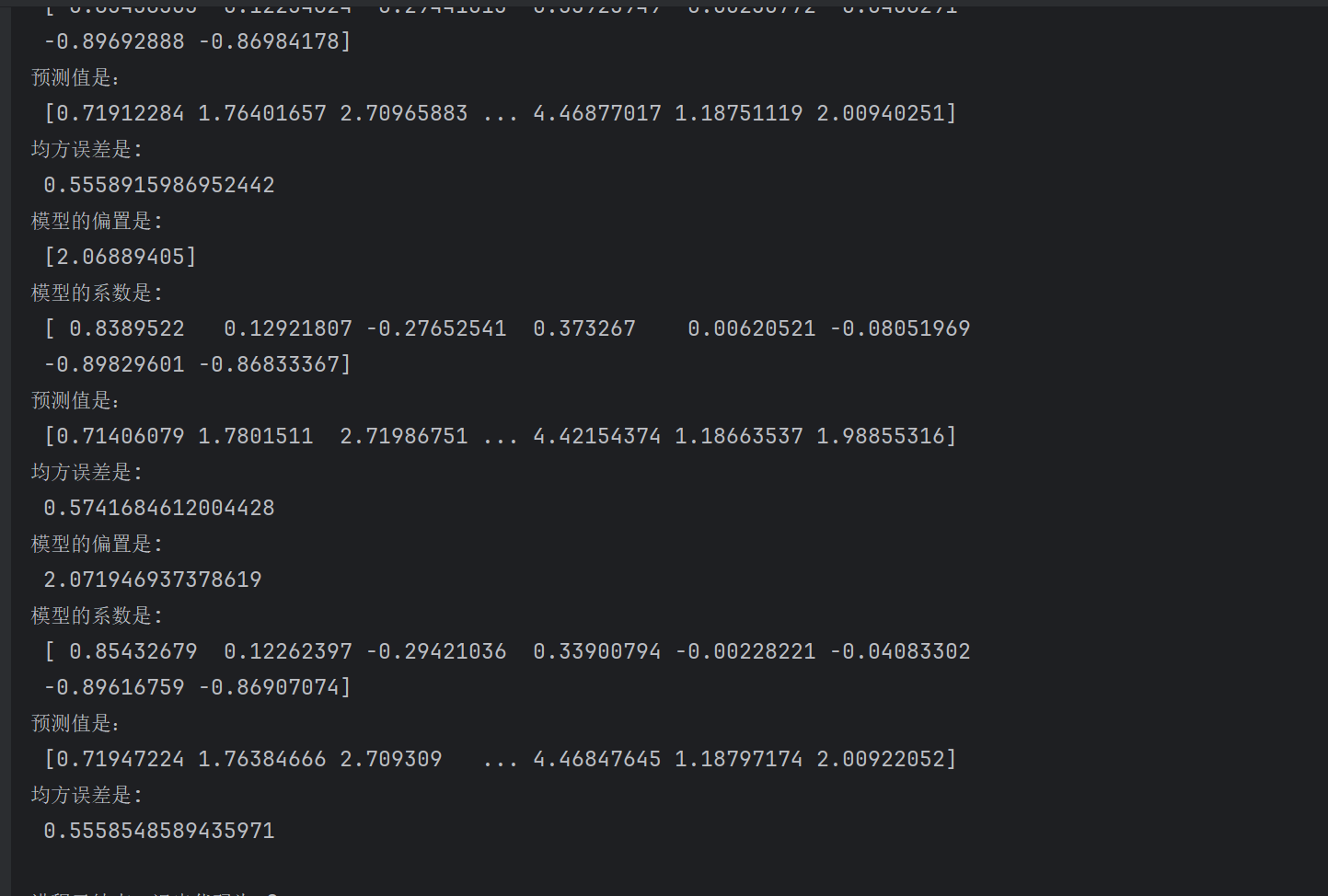
我们发现岭回归是误差是最小的
estimator = RidgeCV(alphas=(0.001,0.01,0.1,1,10,100))
这个是选择一个最优的惩罚力度
11. 模型的保存和加载
11.1 sklearn模型的保存和加载API
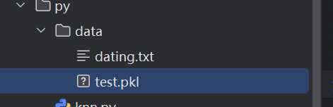
保存:joblib.dump(estimator, 'test.pkl')
加载:estimator = joblib.load('test.pkl')
conda install joblib
import joblib
#岭回归
def linear_model3():# 1. 获取数据housing  = fetch_california_housing()# print(housing)# 2.数据基本处理# 2.1 分割数据x_train, x_test, y_train, y_test = train_test_split(housing.data, housing.target,test_size=0.2,random_state=42)# 3. 特征工程--标准化transfer = StandardScaler()x_train=transfer.fit_transform(x_train)x_test=transfer.transform(x_test)# 4. 机器学习-线性回归# 4.1 estimator = Ridge(alpha=1)estimator = RidgeCV(alphas=(0.001,0.01,0.1,1,10,100))estimator.fit(x_train, y_train)#4.2保存模型joblib.dump(estimator,"./data/test.pkl")print("模型的偏置是:\n",estimator.intercept_)print("模型的系数是:\n",estimator.coef_)# 5. 模型评估#5.1 预测值y_pre=estimator.predict(x_test)print("预测值是:\n",y_pre)#5.2 均方误差mse = mean_squared_error(y_test,y_pre)print("均方误差是:\n",mse)
def linear_model3():# 1. 获取数据housing = fetch_california_housing()# print(housing)# 2.数据基本处理# 2.1 分割数据x_train, x_test, y_train, y_test = train_test_split(housing.data, housing.target,test_size=0.2,random_state=42)# 3. 特征工程--标准化transfer = StandardScaler()x_train=transfer.fit_transform(x_train)x_test=transfer.transform(x_test)# 4. 机器学习-线性回归#4.3 加载模型estimator = joblib.load("./data/test.pkl")print("模型的偏置是:\n",estimator.intercept_)print("模型的系数是:\n",estimator.coef_)# 5. 模型评估#5.1 预测值y_pre=estimator.predict(x_test)print("预测值是:\n",y_pre)#5.2 均方误差mse = mean_squared_error(y_test,y_pre)print("均方误差是:\n",mse)
这样就还是可以使用的