当前位置：首页 > news >正文

Hough Transform 超详细学习笔记

news 2025/9/13 8:40:34

Hough Transform 超详细学习笔记

注意： 使用英文作为章节名，大约 90% 内容为中文。

Image and parameter space

先定义一个工具函数，方便画出网格线和坐标系

import numpy as np
import matplotlib.pyplot as plt
from typing import List, Tuple
from PIL import Image
import cv2def plot_points_and_lines_with_grid(ax: plt.Axes,ax_labels = ["x", "y"],scatter_arg_kwarg_pair: Tuple = None,line_arg_kwarg_pairs: List[Tuple] = None,limits: List[int] = [-5, 5, -5, 5]
):"""_summary_https://stackoverflow.com/questions/13430231/how-i-can-get-cartesian-coordinate-system-in-matplotlibArgs:ax (_type_): _description_scatter_arg_kwarg_pair (Tuple, optional): _description_. Defaults to None.line_arg_kwarg_pairs (List[Tuple], optional): _description_. Defaults to None.label_size (int, optional): _description_. Defaults to 14.Returns:_type_: _description_"""    # Plot pointsif scatter_arg_kwarg_pair is not None:scatter_args, scatter_kwargs = scatter_arg_kwarg_pairax.scatter(*scatter_args, **scatter_kwargs)# Plot linesif line_arg_kwarg_pairs is not None:for line_args, line_kwargs in line_arg_kwarg_pairs:ax.plot(*line_args, **line_kwargs)# Select length of axes and the space between tick labelsxmin, xmax, ymin, ymax = limitsticks_frequency = 1# Set identical scales for both axesax.set(xlim=(xmin-1, xmax+1), ylim=(ymin-1, ymax+1), aspect='equal')# Set bottom and left spines as x and y axes of coordinate systemax.spines['bottom'].set_position('zero')ax.spines['left'].set_position('zero')# Remove top and right spinesax.spines['top'].set_visible(False)ax.spines['right'].set_visible(False)# Create 'x' and 'y' labels placed at the end of the axesax.set_xlabel(ax_labels[0], size=14, labelpad=-24, x=1.03)ax.set_ylabel(ax_labels[1], size=14, labelpad=-21, y=1.02, rotation=0)# Create custom major ticks to determine position of tick labelsx_ticks = np.arange(xmin, xmax+1, ticks_frequency)y_ticks = np.arange(ymin, ymax+1, ticks_frequency)ax.set_xticks(x_ticks[x_ticks != 0])ax.set_yticks(y_ticks[y_ticks != 0])# Create minor ticks placed at each integer to enable drawing of minor grid# lines: note that this has no effect in this example with ticks_frequency=1ax.set_xticks(np.arange(xmin, xmax+1), minor=True)ax.set_yticks(np.arange(ymin, ymax+1), minor=True)# Draw major and minor grid linesax.grid(which='both', color='grey', linewidth=1, linestyle='-', alpha=0.2)return ax

Image Space and Parameter Space

Image space

在 Image Space 中，我们将一条直线表示为：

$y = m x + b$

其中 $m$ 和 $b$ 为 parameters， $x$ 和 $y$ 为 variables

Parameter Space

在 Parameter Space 中，我们将一条直接表示为：

$y - m x = b$

其中 $x$ 和 $y$ 为 parameters， $m$ 和 $b$ 为 variables

def line_image_space(x, m, b):return m * x + bdef line_parameter_space(m, x, y):return y - m * x

A line becomes a point

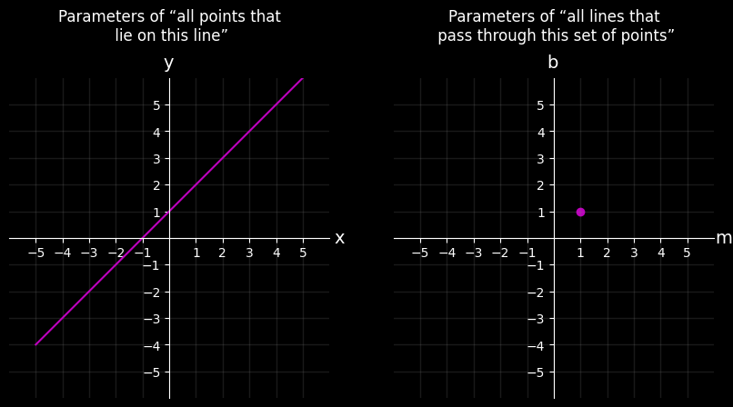
下图中，我们将一个 image space 的直线转化为 parameter space 中的一个点：

Image Space 直线的斜率 m 对应 Parameter Space 中点的横轴坐标 m
Image Space 直线的截距 b 坐标对应 Parameter Space 中点的纵轴坐标 b

nums = np.linspace(-5, 5, 11)fig, ax = plt.subplots(1, 2, figsize=(10, 5))# Plot On Image Space
b = 1
m = 1
x = nums.copy()
y = line_image_space(x, m, b)ax[0].set_title("Parameters of “all points that\n lie on this line”", pad=30)
plot_points_and_lines_with_grid(ax[0],line_arg_kwarg_pairs = [[(x, y), {"color": "m"}]]
)# Plot On Parameter Space
ax[1].set_title("Parameters of “all lines that\n pass through this set of points”", pad = 30)
plot_points_and_lines_with_grid(ax[1],scatter_arg_kwarg_pair = [(), {"x": [m],"y": [b],"c": ["m"],}],ax_labels = ['m', 'b']
)
plt.show()

![[101-Articles/Hough Transform 超详细学习笔记/attachments/hough_transform_7_0.png]]
在这里插入图片描述

A Point becomes a line

回顾 Image Space： $y = m x + b$ ，Parameter Space： $y - m x = b$

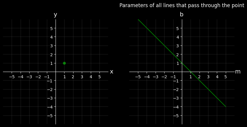
下图中，我们将一个 image space 的点转化为 parameter space 中的一条直线：

Image Space 点的 x 坐标对应 Parameter Space 中直线的斜率 -x，
Image Space 点的 y 坐标变成 Parameter Space 中直线的截距 y

fig, ax = plt.subplots(1, 2, figsize=(10, 5))# Point On Image Space
image_space_point = [1, 1]plot_points_and_lines_with_grid(ax[0],scatter_arg_kwarg_pair = [(), {"x": [image_space_point[0]],"y": [image_space_point[1]],"c": ["g"],}]
)# Line On Parameter Space
m = nums.copy()
x, y = image_space_point
b = line_parameter_space(m, x, y)ax[1].set_title("Parameters of all lines that pass through the point", pad = 30)plot_points_and_lines_with_grid(ax[1],line_arg_kwarg_pairs = [[(m, b), {"color": "g"}]],ax_labels = ['m', 'b']
)plt.show()

在这里插入图片描述

Four points becomes?

回顾 Image Space： $y = m x + b$ ，Parameter Space： $y - m x = b$

下图中，我们将 4 个来自 image space 的点，转换为 parameter space 中的直线

Image Space 点的 x 坐标对应 Parameter Space 中直线的斜率 -x，
Image Space 点的 y 坐标变成 Parameter Space 中直线的截距 y

复核：下图下图绿色的点和直线，左侧 image space 点 [1, -1] 对应右侧 parameter space 直线

斜率为 -x，即 -1
截距为 y，即 1，具体来说右图绿色直线与 b 轴相交于 [0, -1]

fig, ax = plt.subplots(1, 2, figsize=(10, 5))# Plot On Image Space
pts = [[1, 1], [3, 3], [-2, -2], [1, -1]]
colors = ["green", "red", "blue", "yellow"]xs = [pt[0] for pt in pts]
ys = [pt[1] for pt in pts]plot_points_and_lines_with_grid(ax[0],scatter_arg_kwarg_pair = [(), {"x": xs,"y": ys,"c": colors,}]
)# Plot On Parameter Space
# x, y = image_space_pointline_arg_kwarg_pairs = [[(nums.copy(), line_parameter_space(nums.copy(), x, y)), {"color": color}] for x, y, color in zip(xs, ys, colors)]ax[1].set_title("Parameters of all lines that\n pass through these point", pad = 30)
plot_points_and_lines_with_grid(ax[1],line_arg_kwarg_pairs = line_arg_kwarg_pairs,ax_labels = ['m', 'b']
)plt.show()

在这里插入图片描述

Line Detection by Hough Transform

Key idea: points vote for the possible models

Quantize Parameter Space $(m, c)$
Create Accumulator Array $A (m, c)$
Set $\quad \forall m, c$
For each image edge $(xi,yi)\left(x_i, y_i\right)$
- For each element in $A (m, c)$
- If $(m, c)$ lies on the line: $c=-x_i m+y_i$
  - Increment $A (m, c) = A (m, c) + 1$
Find local maxima in $A (m, c)$

遍历边缘图中的点：

参数空间中由 slope $m$ 和 intercept $c$ 组成，构成一条条直线方程
将边缘图中的点的坐标（x,y）代入方程之中，计算 $b = y - m x$
如果 $b$ 与 $c$ 相等，则说明点在直线上，投票 +1

准备宽高为 (11, 11) 的 edge 图，以其中心点为原点，将 [[1, 1], [3, 3], [-2, -2], [1, -1]] 这四个点移动到相应位置

edge_img = np.zeros((11, 11), dtype=np.uint8)
offset = 5
# origin_ij = (5, 5)
pts = [[1, 1], [3, 3], [-2, -2], [1, -1]]
pts = np.array(pts) + 5for i, j in pts:edge_img[i, j] = 255# Image.fromarray(cv2.resize(edge_img, (110, 110), interpolation=cv2.INTER_NEAREST))print(pts.tolist())

[[6, 6], [8, 8], [3, 3], [6, 4]]

移动之后，如下图所示

fig, ax = plt.subplots(figsize=(5, 5))# Plot On Image Space
colors = ["green", "red", "blue", "yellow"]xs = [pt[0] for pt in pts.tolist()]
ys = [pt[1] for pt in pts.tolist()]plot_points_and_lines_with_grid(ax,scatter_arg_kwarg_pair = [(), {"x": xs,"y": ys,"c": colors,}],limits=[0, 10, 0, 10]
)
plt.show()

在这里插入图片描述

实现 hough transform 算法并根据 4 个点，计算出相应的直线

def raw_hough_line_detection(edge_img,m_values,c_values,
):# width, height = edge_img.shapenum_m = len(m_values)num_c = len(c_values)accumulator = np.zeros((num_m, num_c))y_idxs, x_idxs = np.nonzero(edge_img) # (row, col) index to edgesfor x, y in zip(x_idxs, y_idxs):for m_idx, m in enumerate(m_values):for c_idx, c in enumerate(c_values):if np.isclose(c, y - m * x):accumulator[m_idx, c_idx] += 1return accumulator, m_values, c_valuesm_values = np.arange(-5, 5 + 1, 1)
c_values = np.arange(-10, 10 + 1, 1)accumulator, m_values, c_values = raw_hough_line_detection(edge_img, m_values, c_values)idx = np.argmax(accumulator)
row = idx // len(c_values)
col = idx % len(c_values)m, c = m_values[row], c_values[col]print(m, c)

1 0

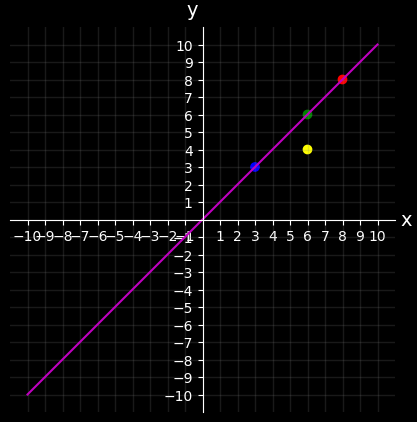
将 4 个点和计算出来的直线画出来

# Plot On Image Space
points = pts.tolist()
colors = ["green", "red", "blue", "yellow"]nums = np.arange(-10, 10+1, 1)xs = [pt[0] for pt in points]
ys = [pt[1] for pt in points]# Plot On Image Space
points = pts.tolist()
colors = ["green", "red", "blue", "yellow"]xs = [pt[0] for pt in points]
ys = [pt[1] for pt in points]nums = np.arange(-10, 10+1, 1)
x = nums.copy()
y = line_image_space(x, m, c)fig, ax = plt.subplots(1, 1, figsize=(5, 5))plot_points_and_lines_with_grid(ax,scatter_arg_kwarg_pair = [(), {"x": xs,"y": ys,"c": colors,}],line_arg_kwarg_pairs = [[(x, y), {"color": "m"}]],limits=[-10, 10, -10, 10]
)plt.show()

在这里插入图片描述

参数空间的问题

$A (m, c)$ 中 $m$ 和 $c$ 的取值范围：

$\begin{align*} -\infty < m < \infty \\ -\infty < c < \infty \end{align*}$

即 $A (m, c)$ 是无限的

Line Parameterizations

Slope intercept form

$y = m x + b$

其中

$m$ 是 slope
$b$ 是 y-intercept

Double intercept form

$\frac{x}{a} + \frac{y}{b} = 1$

其中

$a$ 是 x-intercept
$b$ 是 y-intercept

推导过程：
假设一条直线与 x 轴相交于 $(a, 0)$ ，与 $y$ 轴相交于 $(0, b)$

根据斜率相同，得到

$\frac{y - b}{x - 0}=\frac{y - 0}{x - a}$

然后推导

$\begin{align*} (y-b)(x-a) &= (y-0)(x-0) \\ yx - ya -bx + ba &= yx \\ -ya - bx + ba &= 0 \\ ya + bx &= ba \\ \frac{y}{b} + \frac{x}{a} &= 1 \end{align*}$

最后得到

$\frac{x}{a} + \frac{y}{b} = 1$

Normal form (法线式)

过原点向直线作一垂直线段，若该线长度为 $ρ\rho$ ，且与正 $x$ - 轴的倾斜角为 $θ\theta$ ，则有方程

$\cos \theta + y \sin \theta = \rho$

其中 $cos⁡θ\cos \theta$ 和 $sin⁡θ\sin \theta$ 可以表示为：

$\begin{aligned} \cos \theta & =\frac{\rho}{a} \rightarrow a=\frac{\rho}{\cos \theta} \\ \sin \theta & =\frac{\rho}{b} \rightarrow b=\frac{\rho}{\sin \theta} \end{aligned}$

将其代入 $xa+yb=1\frac{x}{a} + \frac{y}{b} = 1$ ，可得

$\cos \theta + y \sin \theta = \rho$

Better Parameterization

Use normal form:

$\cos \theta+y \sin \theta=\rho$

Given points $(xi,yi)\left(x_i, y_i\right)$ find $(ρ,θ)(\rho, \theta)$ that describe all lines that can pass through this point.

What is the range of $ρ,θ\rho, \theta$ ?

$\begin{aligned} & 0 \leq \theta \leq 2 \pi \\ & 0 \leq \rho \leq \rho_{\max} \end{aligned}$

实际应用中

可以限定 $θ\theta$ 的取值为 $[0,π][0,\pi]$ ，即可，因为 $θ\theta$ 和 $θ+π\theta + \pi$ 是同一直线角度的 2 种表述
$ρmax⁡\rho_{\max}$ 由图片大小决定，为其对角线的长度： $x2+y2\sqrt{x^2 + y^2}$ 。

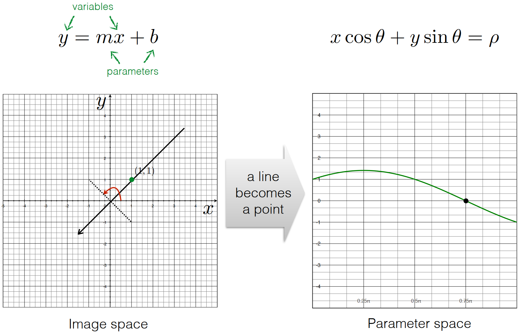
Image Space and Parameter Space (Normal form)

在 Image Space 中，我们将一条直线表示为：

$y = m x + b$

其中 $m$ 和 $b$ 为 parameters， $x$ 和 $y$ 为 variables

在 Parameter Space 中，我们将一条直线表示为法线式：

$\cos \theta+y \sin \theta=\rho$

变量 $x$ 和 $y$ 为 parameters, $θ\theta$ 和 $ρ\rho$ 为 variables

def normal_form_line_parameter_space(theta, x, y):return x * np.cos(theta) + y * np.sin(theta)

增加适用于法线式直线表达的方便画网格的函数

def plot_points_and_lines_with_grid_theta_rho(ax: plt.Axes,ax_labels = [r"$\theta$", r"$\rho$"],scatter_arg_kwarg_pair: List = None,line_arg_kwarg_pairs: List[List] = None,limits: List[int] = [-0.05 * np.pi, np.pi, -4.5, 4.5]
):"""_summary_https://stackoverflow.com/questions/13430231/how-i-can-get-cartesian-coordinate-system-in-matplotlibArgs:ax (_type_): _description_scatter_arg_kwarg_pair (Tuple, optional): _description_. Defaults to None.line_arg_kwarg_pairs (List[Tuple], optional): _description_. Defaults to None.label_size (int, optional): _description_. Defaults to 14.Returns:_type_: _description_"""# Plot pointsif scatter_arg_kwarg_pair is not None:scatter_args, scatter_kwargs = scatter_arg_kwarg_pairax.scatter(*scatter_args, **scatter_kwargs)# Plot linesif line_arg_kwarg_pairs is not None:for line_args, line_kwargs in line_arg_kwarg_pairs:ax.plot(*line_args, **line_kwargs)# Set bottom and left spines as x and y axes of coordinate system# ax.spines['bottom'].set_position('zero')ax.spines['left'].set_position('zero')# Remove top and right spinesax.spines['top'].set_visible(False)ax.spines['right'].set_visible(False)# Select length of axes and the space between tick labelsxmin, xmax, ymin, ymax = limitsticks_frequency = 1# Set identical scales for both axesax.set(xlim=(xmin, xmax), ylim=(ymin, ymax), aspect='auto')# # Create 'x' and 'y' labels placed at the end of the axesax.set_xlabel(ax_labels[0], size=14, labelpad=-24, x=1.03)ax.set_ylabel(ax_labels[1], size=14, labelpad=-21, y=1.02, rotation=0)# # Create custom major ticks to determine position of tick labelsy_ticks = np.arange(int(ymin), int(ymax)+1, ticks_frequency)ax.set_yticks(y_ticks)x_tick = np.arange(0, 1, 0.25)x_tick_labels = [ r"$0$", r"$0.25\pi$",  r"$0.5\pi$", r"$0.75\pi$"]ax.set_xticks(x_tick*np.pi)ax.set_xticklabels(x_tick_labels, fontsize=14)ax.grid(which='both', color='grey', linewidth=1, linestyle='-', alpha=0.2)return ax

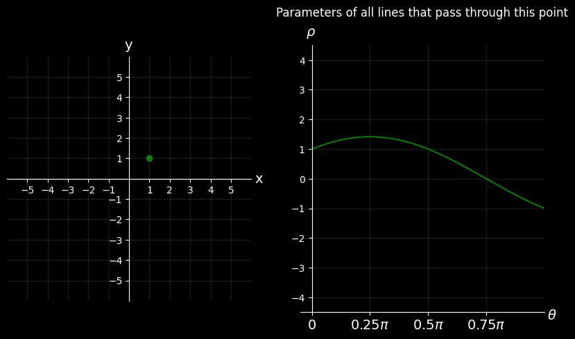
A point becomes a wave

对于点 $(1, 1)$ ，寻找所有经过该点的直线

fig, ax = plt.subplots(1,2, figsize=(10, 5))# Point On Image Space
image_space_point = [1, 1]plot_points_and_lines_with_grid(ax[0],scatter_arg_kwarg_pair = [(), {"x": [image_space_point[0]],"y": [image_space_point[1]],"c": ["g"],}]
)# Line on Parameter Space
degrees = np.arange(0, 180, 1)
thetas = np.deg2rad(degrees)rhos = normal_form_line_parameter_space(thetas, 1, 1)ax[1].set_title("Parameters of all lines that pass through this point", pad=30)plot_points_and_lines_with_grid_theta_rho(ax[1],line_arg_kwarg_pairs=[[(thetas, rhos), {"color": "g"}]]
)plt.show()

在这里插入图片描述

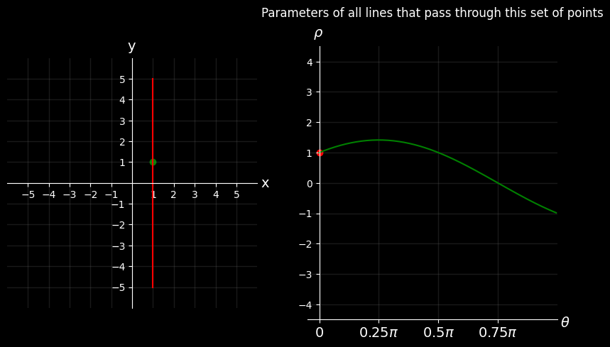
A line becomes a point (1)

对于直线 $x = 1$ （方向为向上），过原点向其作一垂直线段：

与原点的距离（线段长度）： $ρ=1\rho = 1$
线段与 $x$ 轴的夹角为 $θ=0\theta = 0$

fig, ax = plt.subplots(1,2, figsize=(10, 5))# Point On Image Space
image_space_point = [1, 1]xs = np.repeat(1, repeats=11)
ys = np.arange(-5, 5+1, 1)plot_points_and_lines_with_grid(ax[0],scatter_arg_kwarg_pair = [(), {"x": [image_space_point[0]],"y": [image_space_point[1]],"c": ["g"],}],line_arg_kwarg_pairs=[[(xs, ys), {"color": "r"}]]
)# Plot on Parameter Spacedegrees = np.arange(0, 180, 1)
line_thetas = np.deg2rad(degrees)line_rhos = normal_form_line_parameter_space(line_thetas, 1, 1)rho = 1
theta = 0ax[1].set_title("Parameters of all lines that pass through this set of points", pad=30)plot_points_and_lines_with_grid_theta_rho(ax[1],scatter_arg_kwarg_pair = [(), {"x": [theta],"y": [rho],"c": ["r"],}],line_arg_kwarg_pairs=[[(line_thetas, line_rhos), {"color": "g"}]]
)plt.show()

在这里插入图片描述

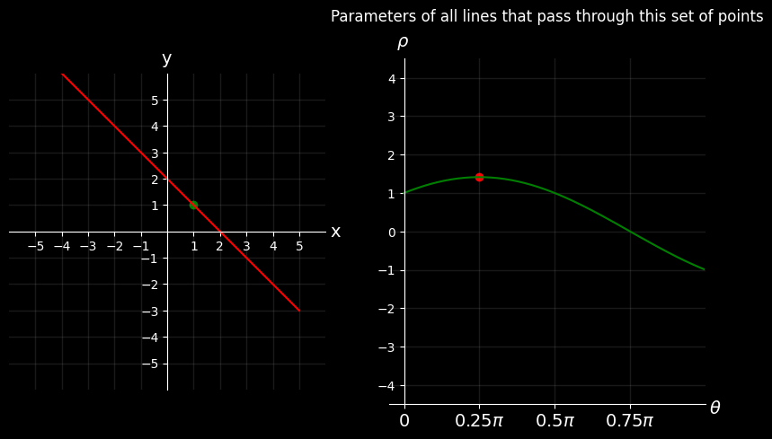
A line becomes a point (2)

对于直线 $x = - x + 2$ ，过原点向其作一垂直线段：

与原点的距离（线段长度）： $ρ=12+12\rho=\sqrt{1^2 + 1^2}$
线段与 $x$ 轴的夹角为 $45$ 度，或者说是 $θarccos⁡1ρ\theta \arccos \frac{1}{\rho}$

fig, ax = plt.subplots(1,2, figsize=(10, 5))# Point On Image Space
image_space_point = [1, 1]xs = np.arange(-5, 5 + 1, 1)
m = -1
b = 2
ys = line_image_space(xs, m, b)plot_points_and_lines_with_grid(ax[0],scatter_arg_kwarg_pair = [(), {"x": [image_space_point[0]],"y": [image_space_point[1]],"c": ["g"],}],line_arg_kwarg_pairs=[[(xs, ys), {"color": "r"}]]
)# Plot on Parameter Spacedegrees = np.arange(0, 180, 1)
line_thetas = np.deg2rad(degrees)
line_rhos = normal_form_line_parameter_space(line_thetas, 1, 1)rho = np.sqrt(1**2 + 1 **2)
theta = np.arccos(1/rho)ax[1].set_title("Parameters of all lines that pass through this set of points", pad=30)plot_points_and_lines_with_grid_theta_rho(ax[1],scatter_arg_kwarg_pair = [(), {"x": [theta],"y": [rho],"c": ["r"],}],line_arg_kwarg_pairs=[[(line_thetas, line_rhos), {"color": "g"}]]
)plt.show()

在这里插入图片描述

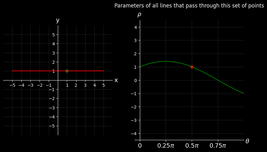
A line becomes a point (3)

对于直线 $y = 1$ ，过原点向其作一垂直线段：

与原点的距离（线段长度）： $ρ=1\rho=1$
线段与 $x$ 轴的夹角为 $90$ 度，或者说是 $θ=arccos⁡01\theta = \arccos \frac{0}{1}$ ，使用 Python 计算 np.deg2rad(90) == np.arccos(0)

fig, ax = plt.subplots(1,2, figsize=(10, 5))# Point On Image Space
image_space_point = [1, 1]xs = np.arange(-5, 5 + 1, 1)
ys = line_image_space(xs, 0, 1)plot_points_and_lines_with_grid(ax[0],scatter_arg_kwarg_pair = [(), {"x": [image_space_point[0]],"y": [image_space_point[1]],"c": ["g"],}],line_arg_kwarg_pairs=[[(xs, ys), {"color": "r"}]]
)# Plot on Parameter Spacedegrees = np.arange(0, 180, 1)
line_thetas = np.deg2rad(degrees)
line_rhos = normal_form_line_parameter_space(line_thetas, 1, 1)rho = 1
theta = np.arccos(0/rho)ax[1].set_title("Parameters of all lines that pass through this set of points", pad=30)plot_points_and_lines_with_grid_theta_rho(ax[1],scatter_arg_kwarg_pair = [(), {"x": [theta],"y": [rho],"c": ["r"],}],line_arg_kwarg_pairs=[[(line_thetas, line_rhos), {"color": "g"}]]
)plt.show()

在这里插入图片描述

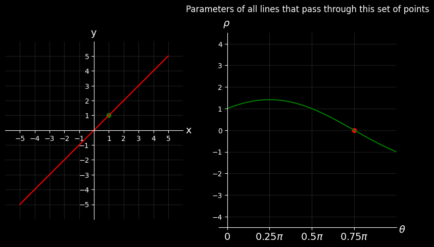
A line becomes a point (4)

对于直线 $y = x$ ，过原点向其作一垂直线段：

与原点的距离（线段长度）： $ρ=0\rho=0$
垂直线段经过点 $(- 1, - 1)$ ，与 $x$ 轴的夹角为 $θ=arccos⁡−112+12\theta = \arccos \frac{-1}{1^2 + 1^2}$

fig, ax = plt.subplots(1,2, figsize=(10, 5))# Point On Image Space
image_space_point = [1, 1]xs = np.arange(-5, 5 + 1, 1)
ys = line_image_space(xs, 1, 0)plot_points_and_lines_with_grid(ax[0],scatter_arg_kwarg_pair = [(), {"x": [image_space_point[0]],"y": [image_space_point[1]],"c": ["g"],}],line_arg_kwarg_pairs=[[(xs, ys), {"color": "r"}]]
)# Plot on Parameter Spacedegrees = np.arange(0, 180, 1)
line_thetas = np.deg2rad(degrees)
line_rhos = normal_form_line_parameter_space(line_thetas, 1, 1)rho = 0
theta = np.arccos(-1/np.sqrt(1**2 + 1**2))ax[1].set_title("Parameters of all lines that pass through this set of points", pad=30)plot_points_and_lines_with_grid_theta_rho(ax[1],scatter_arg_kwarg_pair = [(), {"x": [theta],"y": [rho],"c": ["r"],}],line_arg_kwarg_pairs=[[(line_thetas, line_rhos), {"color": "g"}]]
)plt.show()

在这里插入图片描述

关于如何在上图画出垂直线段，参考下图：

在这里插入图片描述

Why $ρ\rho$ is negative?

在这里插入图片描述

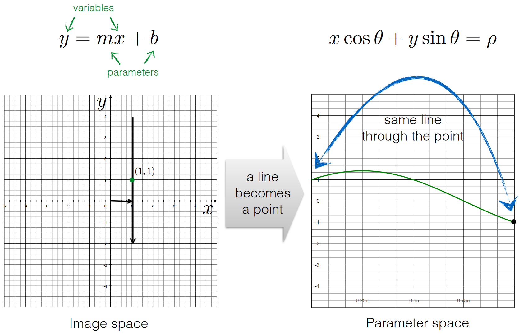
上图中的右图，点 $(θ=0,ρ=1)(\theta = 0, \rho = 1)$ 和点 $(θ=π,ρ=−1(\theta = \pi, \rho = -1$ ) 表示同一条直线； $ρ\rho$ 为负数是因为方向不同，造成的 $θ\theta$ 值不同，从而导致 $ρ\rho$ 符号变化，具体见：

在这里插入图片描述

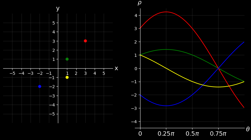
Four lines becomes?

fig, ax = plt.subplots(1,2, figsize=(10, 5))# Point On Image Space
image_space_point = [1, 1]# Plot On Image Space
pts = [[1, 1], [3, 3], [-2, -2], [1, -1]]
colors = ["green", "red", "blue", "yellow"]xs = [pt[0] for pt in pts]
ys = [pt[1] for pt in pts]plot_points_and_lines_with_grid(ax[0],scatter_arg_kwarg_pair = [(), {"x": xs,"y": ys,"c": colors,}],
)# Plot on Parameter Spacedegrees = np.arange(0, 180, 1)
thetas = np.deg2rad(degrees)line_arg_kwarg_pairs = [[(thetas.copy(), normal_form_line_parameter_space(thetas.copy(), x, y)), {"color": color}] for x, y, color in zip(xs, ys, colors)]plot_points_and_lines_with_grid_theta_rho(ax[1],line_arg_kwarg_pairs=line_arg_kwarg_pairs
)plt.show()

在这里插入图片描述

实现

Initialize accumulator H to all zeros
For each edge point $(x, y)$ in the image
- For $θ=0\theta=0$ to 180
  - $ρ=xcos⁡θ+ysin⁡θ\rho=x \cos \theta+y \sin \theta$
  - $H(θ,ρ)=H(θ,ρ)+1H(\theta, \rho)=H(\theta, \rho)+1$
- end
  end
Find the value(s) of $(θ,ρ)(\theta, \rho)$ where $H(θ,ρ)H(\theta, \rho)$ is a local maximum
The detected line in the image is given by $ρ=xcos⁡θ+ysin⁡θ\rho=x \cos \theta+y \sin \theta$

以下是来自 https://alyssaq.github.io/2014/understanding-hough-transform/ 的实现

## Implementationimport numpy as npdef hough_line_np(img):# Rho and Theta rangesthetas = np.deg2rad(np.arange(-90.0, 90.0))width, height = img.shapediag_len = int(np.ceil(np.sqrt(width * width + height * height)))   # max_distrhos = np.linspace(-diag_len, diag_len, diag_len * 2)# Cache some resuable valuescos_t = np.cos(thetas)sin_t = np.sin(thetas)num_thetas = len(thetas)# Hough accumulator array of theta vs rhoaccumulator = np.zeros((2 * diag_len, num_thetas), dtype=np.uint64)y_idxs, x_idxs = np.nonzero(img)  # (row, col) indexes to edges# Vote in the hough accumulatorfor i in range(len(x_idxs)):x = x_idxs[i]y = y_idxs[i]for t_idx in range(num_thetas):# Calculate rho. diag_len is added for a positive indexrho = round(x * cos_t[t_idx] + y * sin_t[t_idx]) + diag_lenaccumulator[rho, t_idx] += 1return accumulator, thetas, rhos## Usage# Create binary image and call hough_line
image = np.zeros((50,50))
image[10:40, 10:40] = np.eye(30)
accumulator, thetas, rhos = hough_line_np(image)# Easiest peak finding based on max votes
idx = np.argmax(accumulator)
rho = rhos[int(idx / accumulator.shape[1])]
theta = thetas[idx % accumulator.shape[1]]
print("rho={0:.2f}, theta={1:.0f}".format(rho, np.rad2deg(theta)))

rho=0.50, theta=-45

使用 OpenCV

img = np.zeros((192, 192), dtype=np.uint8)points = [[100, 100], [120, 120], [150, 150], [180, 180], [142, 23]]for i, j in points:img[i, j] = 255Image.fromarray(img)

在这里插入图片描述

lines = cv2.HoughLines(img, 1, np.pi / 180, 2)cdst = img.copy()# Draw the lines
if lines is not None:for i in range(0, len(lines)):rho = lines[i][0][0]theta = lines[i][0][1]print(theta, rho)a = np.cos(theta)b = np.sin(theta)x0 = a * rhoy0 = b * rhopt1 = (int(x0 + 1000*(-b)), int(y0 + 1000*(a)))pt2 = (int(x0 - 1000*(-b)), int(y0 - 1000*(a)))cv2.line(cdst, pt1, pt2, (255,255,255), 1, cv2.LINE_AA)Image.fromarray(cdst)

2.3561945 0.0

在这里插入图片描述

上面的代码中

$\cos \theta \\ b = \sin \theta$

其中，根据定义，向量 $(a, b)$ 与直线构建的向量是垂直的，那么直线可以表示为 $v = (- b, a)$ 的向量（相乘为 0）。

根据直线公式公式

$\mathbf{r} = \mathbf{r}_0 + t \mathbf{v}$

上面的代码中 pt1 和 pt2 分别为 $t = 1000$ 和 $t = - 1000$ 时计算的

使用 scikit-image

from skimage.transform import hough_line, hough_line_peaks
hspace, angles, dists = hough_line(img)
hspace, angles, dists = hough_line_peaks(hspace, angles, dists)img_display = img.copy()for _, angle, dist in zip(hspace, angles, dists):a = np.cos(angle)b = np.sin(angle)(x0, y0) = dist * np.array([a, b])pt1 = (int(x0 + 1000*(-b))), int(y0 + 1000*(a))pt2 = (int(x0 - 1000*(-b))), int(y0 - 1000*(a))cv2.line(img_display, pt1, pt2, (255,255,255), 1, cv2.LINE_AA)Image.fromarray(img_display)

在这里插入图片描述

参考资料

https://www.cs.cmu.edu/~16385/s17/Slides/5.3_Hough_Transform.pdf
https://alyssaq.github.io/2014/understanding-hough-transform/
https://gist.github.com/bygreencn/6a900fd2ff5d0101473acbc3783c4d92
https://docs.opencv.org/4.x/d9/db0/tutorial_hough_lines.html
https://scikit-image.org/docs/stable/auto_examples/edges/plot_line_hough_transform.html