数学建模：智能优化算法

前言

有点意思吼。

一、粒子群算法（PSO）

1.基本概念

首先，需要明确“群体智能”这个概念。群体智能就是群体动物或昆虫的集体行为，比如蚂蚁，鸟群，鱼群等，核心思路就是通过模拟这些群体的行为来对问题进行优化的。

粒子群算法模拟的是鸟群捕食的算法，将一只鸟看作一个粒子。过程就是将要求解的最优解看作食物最多的位置，然后每只鸟都会根据自己的经验，即个体最优解，和其他鸟的经验，即群体最优解，来决定下一步的飞行方向，从而避免去到虽然离得近，但食物较少的局部最优解，而是快速找到食物最多的位置。

假设要搜索的空间是D维的，即要优化的变量有D个，一共有m个粒子。初始时，随机将这m个粒子洒在地图上，那么每个粒子都会有自己的坐标向量X，还会有自己的飞翔速度向量V，表示下一步要去的方向和飞行速度。那么在整个地图中，每个粒子都会有一个自己搜索到的个体最优位置P，还有整个粒子群要去到的整体最优位置G。还有，为了量化每个位置的好坏，还需要设置适应度函数来评价每个位置的好坏。

那么迭代更新的策略是，每个粒子下一步的飞翔速度向量V，等于惯性权重w乘以上一步的飞翔速度向量，表示对上一代的继承程度，再加上加速常数c1，表示每次粒子向个体最优位置移动的步长，乘以随机数r1再乘以在第i个方向上，个体最优位置p减去当前位置x之差，再加上c2乘以随机数r2再乘以在第i个方向上，整体最优位置g减去当前位置x之差。即：

可以发现，该公式由三个部分组成，分别表示对之前速度的继承，自己的经验和群体的经验。哪一部分越大，表示对哪一部分越重视，或者说越相信。通常情况下，c1和c2都取2即可。

所以，下一步的坐标就是当前坐标加上下一步的速度向量。

 2.基本步骤

首先就是随机在地图上洒下m个粒子，初始化每个粒子的个体最优就是自己所在的位置，整体最优为所有个体最优中适应度最好的那个位置。其中，一般粒子数m取20到40，对于一些较难的问题也可以取到100到200。此外，为了限制飞翔速度，所以还要设置粒子的最大速度，一般是整个空间的可行范围的长度乘以一个0.1到0.5之间的小数。当然，由于速度越大越利于全局搜索，也可以设置随着迭代加深最大速度逐渐减小。又因为对于惯性权重w，从物理的角度理解，惯性越大越容易往前冲，所以w越大越利于全局搜索，越小越利于算法收敛，所以实际情况中一般选择随着迭代加深线性地减小w的值。其中线性公式一般为最大权重减去最大权重减最小权重的差除以最大迭代次数乘以当前迭代次数，即：

之后在迭代的过程中，每次遍历所有粒子，计算新位置的适应度，看能否更新个体最优位置，之后再看所有新的个体最优位置能否更新整体最优位置。

最后，当达到了限制的迭代次数，或者整体最优的适应度变化小于了某个阈值或达到了需要的适应度，那么就可以停止了。

3.练习

import numpy as np
import matplotlib.pyplot as plt
from matplotlib.animation import FuncAnimation
#使用中文字体
from matplotlib.pylab import mpl
mpl.rcParams['font.sans-serif'] = ['SimHei']
mpl.rcParams['axes.unicode_minus'] = False#目标函数：Rastrigin Function（多峰函数，全局最小值在原点0处）
def rastrigin(x):A = 10return A * len(x) + sum([(xi ** 2 - A * np.cos(2 * np.pi * xi)) for xi in x])class ParticleSwarmOptimizer:def __init__(self, objective_func, n_particles, dimensions, bounds, w=0.7, c1=2, c2=2):"""粒子群优化算法初始化:param objective_func: 目标函数:param n_particles: 粒子数量:param dimensions: 变量维度:param bounds: 每个维度的边界 [min, max]:param w: 惯性权重:param c1: 个体学习因子:param c2: 社会学习因子"""self.objective_func = objective_funcself.n_particles = n_particlesself.dimensions = dimensionsself.bounds = np.array(bounds)self.w = wself.c1 = c1self.c2 = c2#初始化粒子位置和速度self.positions = np.random.uniform(low=bounds[0], high=bounds[1],size=(n_particles, dimensions))self.velocities = np.zeros((n_particles, dimensions))#个体最优位置和全局最优位置self.pbest_positions = self.positions.copy()self.pbest_scores = np.full(n_particles, float('inf'))self.gbest_position = Noneself.gbest_score = float('inf')#初始化个体最优和全局最优for i in range(n_particles):score = objective_func(self.positions[i])self.pbest_scores[i] = scoreif score < self.gbest_score:self.gbest_score = scoreself.gbest_position = self.positions[i].copy()#记录历史最优值self.history = []def update(self):"""更新粒子位置和速度"""for i in range(self.n_particles):#更新速度r1, r2 = np.random.rand(2)cognitive = self.c1 * r1 * (self.pbest_positions[i] - self.positions[i])social = self.c2 * r2 * (self.gbest_position - self.positions[i])self.velocities[i] = self.w * self.velocities[i] + cognitive + social#更新位置self.positions[i] += self.velocities[i]#边界处理self.positions[i] = np.clip(self.positions[i], self.bounds[0], self.bounds[1])#计算新位置的适应度current_score = self.objective_func(self.positions[i])#更新个体最优if current_score < self.pbest_scores[i]:self.pbest_scores[i] = current_scoreself.pbest_positions[i] = self.positions[i].copy()#更新全局最优if current_score < self.gbest_score:self.gbest_score = current_scoreself.gbest_position = self.positions[i].copy()self.history.append(self.gbest_score)def optimize(self, max_iter=100):"""执行优化"""for _ in range(max_iter):self.update()return self.gbest_position, self.gbest_score#参数设置
n_particles = 30 #粒子数
dimensions = 2 #维度
bounds = [-5.12, 5.12]  #Rastrigin函数的典型搜索范围
max_iter = 100 #最大迭代次数#执行优化
pso = ParticleSwarmOptimizer(rastrigin, n_particles, dimensions, bounds)
best_position, best_score = pso.optimize(max_iter)#输出结果
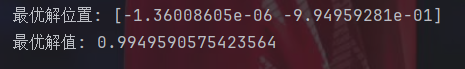
print(f"最优解位置: {best_position}")
print(f"最优解值: {best_score}")#绘制收敛曲线
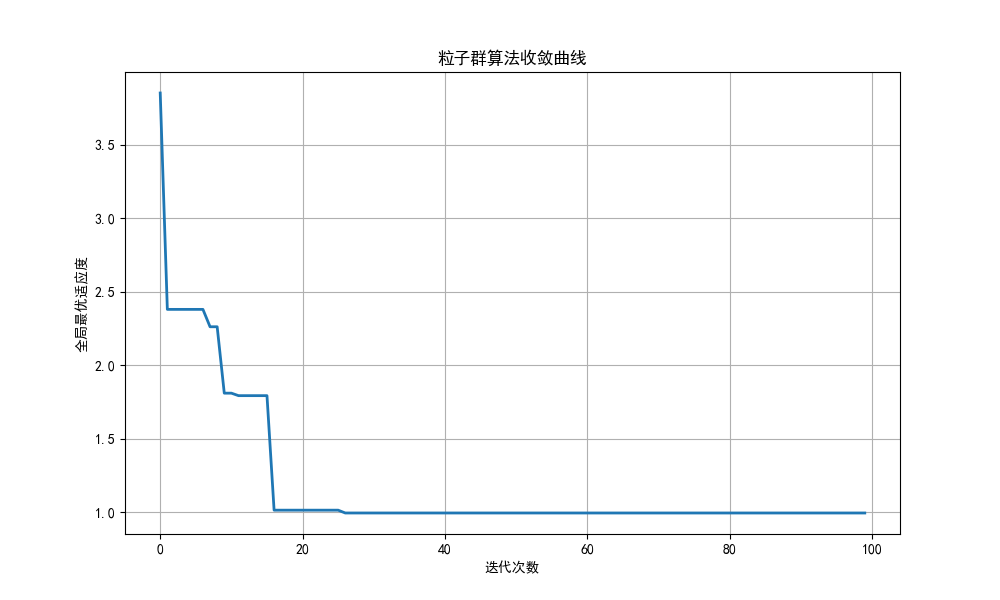
plt.figure(figsize=(10, 6))
plt.plot(pso.history, linewidth=2)
plt.title('粒子群算法收敛曲线')
plt.xlabel('迭代次数')
plt.ylabel('全局最优适应度')
plt.grid(True)
plt.show()#创建动态搜索过程可视化
if dimensions == 2:fig, ax = plt.subplots(figsize=(10, 8))#准备函数等高线x = np.linspace(bounds[0], bounds[1], 100)y = np.linspace(bounds[0], bounds[1], 100)X, Y = np.meshgrid(x, y)Z = np.zeros_like(X)for i in range(X.shape[0]):for j in range(X.shape[1]):Z[i, j] = rastrigin([X[i, j], Y[i, j]])#绘制等高线contour = ax.contourf(X, Y, Z, 50, cmap='viridis')plt.colorbar(contour)ax.set_title('粒子群算法搜索过程')ax.set_xlabel('x1')ax.set_ylabel('x2')#初始化粒子位置particles = ax.scatter([], [], c='white', edgecolor='black', s=80, alpha=0.7, label='粒子位置')global_best = ax.scatter([], [], c='red', s=150, marker='*', label='全局最优')#迭代次数iter_text = ax.text(0.02, 0.95, '', transform=ax.transAxes,fontsize=14, color='white',bbox=dict(facecolor='black', alpha=0.5, edgecolor='none'))#适应度值fitness_text = ax.text(0.02, 0.90, '', transform=ax.transAxes,fontsize=12, color='white',bbox=dict(facecolor='black', alpha=0.5, edgecolor='none'))#迭代状态status_text = ax.text(0.98, 0.02, '', transform=ax.transAxes,fontsize=12, color='white', ha='right',bbox=dict(facecolor='black', alpha=0.5, edgecolor='none'))#图例ax.legend(loc='upper right')#创建pso_anim = ParticleSwarmOptimizer(rastrigin, n_particles, dimensions, bounds)#动画更新函数def update(frame):#更新迭代次数current_iter = min(frame, max_iter)iter_text.set_text(f'迭代次数: {current_iter}/{max_iter}')if frame <= max_iter:#在达到最大迭代次数前继续更新if frame > 0:  #第0帧显示初始状态，不需要更新pso_anim.update()#更新粒子位置particles.set_offsets(pso_anim.positions)#更新全局最优位置global_best.set_offsets([pso_anim.gbest_position])#更新适应度fitness_text.set_text(f'全局最优适应度: {pso_anim.gbest_score:.6f}')#更新状态if frame < max_iter:status_text.set_text('优化中...')else:status_text.set_text('优化完成')#返回所有需要重绘的对象return particles, global_best, iter_text, fitness_text, status_text#创建动画#设置总帧数为max_iter + 50 -> 50帧用于显示定格效果total_frames = max_iter + 50ani = FuncAnimation(fig, update, frames=total_frames, interval=200,blit=True, repeat=False)plt.show()

整体代码的思路就是构建一个粒子群算法类，里面包括初始化，更新和优化三个方法。其中，优化方法会重复调用更新方法，最终返回全局最优的点和全局最优位置的适应度。

动图放不出来就不放了（）

二、遗传算法（GA）

1.基本概念

因为名字就叫“遗传算法”，所以肯定是和遗传有点关系。

首先，需要明确染色体和基因的概念。染色体就是个体的某种字符串或数组形式的编码表示，字符串中的每个字符就是基因。举个例子，对于个体9，如果选择用二进制编码进行表示，那它的染色体就是1001，其中的每个字符就是它的基因。再举个例子，在TSP问题中，每个个体的编码可以是由先后走过的节点编号组成的数组。

之后，有了染色体和基因，就可以进行遗传了。遗传就是关于染色体的运算，一共有三种操作，分别是选择，交叉和变异。选择很好理解，就是模拟自然选择，即适应度高的个体有更大的概率被选中进行繁殖。交叉就是模拟被选中的父代个体交换部分染色体信息，从而产生新的子代个体。变异就是模拟新产生的子代以较小的概率随机改变染色体上的某些部分，为整个种群引入新的可能性，避免陷入局部最优。

2.基本步骤

首先，和粒子群算法类似，初始随机生成一个种群，然后计算每个个体的适应度。之后，每次迭代时先执行选择操作，选出若干个父代。然后让父代两两配对去生成子代，过程中对子代执行交叉和变异操作。最后让新生成的子代加入之前的种群，并以一定策略进行淘汰。当达到最大迭代次数，或适应度最大的个体的适应度达到了要求，再或者连续几次迭代最优适应度都没产生明显变化，那就可以停止迭代了。

细节上，首先是编码方式的选择。一般来讲，如果是求解一个规划函数在某个范围上的最值，那么此时就可以用二进制编码，表示个体的x值。而如果是TSP问题，就可以是先后到达的节点编号。如果是01背包问题，那就可以是0或1构成的数组，表示要或不要。

在选择的过程中，一般有三种策略，分别是轮盘赌选择，排序选择和锦标赛选择。轮盘赌选择就是先求出所有个体的总适应度，然后设定每个个体被选中的概率为自己的适应度除以总适应度。之后按这个概率循环，直到选出若干个作为父代。排序选择就是先对所有个体按适应度排序，之后根据排序的名次从大到小分配从高到低的概率，然后同样循环选择。锦标赛选择就是每次随机选择k个个体，比较这k个个体的适应度，其中适应度最大的胜出。之后同样进行循环选择，注意这里胜出的个体一般会选择放回重新参与比赛。注意，这三种选择方式都可以保证同一个个体可以被多次选中参与繁殖，以此来模拟自然界中适应度高的个体往往有更多的繁殖机会，从而更能把优秀的基因传递下去。

交叉操作首先要有一个交叉概率，即每个子代是否进行交叉。如果是二进制编码，可以考虑先随机选择一个交叉点，划分两个父代的字符串，然后拼接产生父a1+父b2和父b1+父a2两个子代。如果是TSP问题，那么可以在父代1中先随机选择两个交叉点，然后把这两个交叉点内的数字直接抄到子代的相同位置处。接着，在父代2中从右侧的交叉点开始，循环遍历，将没填过的数字抓出来，按遍历到的顺序填到子代剩余的位置即可。而对于没被选中交叉的子代，直接复制父代的染色体即可。

变异操作也有一个变异率，但这个概率就非常小了，一般是0.0001到0.1之间。对于二进制编码，可以直接随机一个位置将状态取反。对于TSP问题，可以随机两个位置交换。对于实数编码，可以考虑随机一个位置加上一个微小的扰动，改变其数值大小。

3.练习

import numpy as np#遗传算法参数
POP_SIZE = 10  #种群大小
DNA_SIZE = 10  #染色体长度（2^10=1024，可表示0-1023）
CROSS_RATE = 0.8  #交叉概率
MUTATION_RATE = 0.1  #变异概率
N_GENERATIONS = 20  #迭代代数
X_BOUND = [0, 1023]  #x的取值范围#适应度函数(目标函数)
def F(x):return x ** 2#生成个体染色体 -> 二进制编码
def create_individual():return np.random.randint(2, size=DNA_SIZE)#生成初始种群
def create_population():return [create_individual() for _ in range(POP_SIZE)]#染色体解码 -> 二进制转十进制
def translateDNA(pop):return np.array([individual.dot(2 ** np.arange(DNA_SIZE)) for individual in pop])#计算适应度
def get_fitness(pop):x = translateDNA(pop)pred = F(x)#将最小适应度变成0，防止出现负数#再加上一个小数，避免在轮盘赌里被完全忽略return (pred - np.min(pred)) + 1e-3#选择操作 -> 轮盘赌
def select(pop, fitness):idx = np.random.choice(np.arange(POP_SIZE), size=POP_SIZE, replace=True,p=fitness / fitness.sum())return [pop[i] for i in idx]#交叉操作 -> 单点交叉
def crossover(parent1, parent2):if np.random.rand() < CROSS_RATE:#随机选择交叉点cross_point = np.random.randint(1, DNA_SIZE)#创建子代child = np.concatenate((parent1[:cross_point], parent2[cross_point:]))return childreturn parent1.copy()  #返回父代副本#变异操作 -> 位翻转
def mutate(child):#避免修改原对象mutated = child.copy()for point in range(DNA_SIZE):if np.random.rand() < MUTATION_RATE:mutated[point] = mutated[point]^1  #位翻转return mutated#遗传算法流程
def genetic_algorithm():#初始化种群pop = create_population()best_fitness_history = []  #记录每代最佳适应度for generation in range(N_GENERATIONS):#计算适应度fitness = get_fitness(pop)#记录并打印当前最优解best_idx = np.argmax(fitness)best_individual = pop[best_idx]best_x = translateDNA([best_individual])[0]best_fitness = F(best_x)best_fitness_history.append(best_fitness)print(f"迭代数： {generation + 1}: x = {best_x}, f(x) = {best_fitness}")#选择操作selected_pop = select(pop, fitness)#创建新种群new_pop = []#保留最优个体new_pop.append(best_individual.copy())#生成子代for i in range(POP_SIZE - 1):  # size-1 -> 因为已经保留了一个精英#随机选择两个父代idx1, idx2 = np.random.choice(POP_SIZE, size=2, replace=False)parent1 = selected_pop[idx1]parent2 = selected_pop[idx2]#交叉child = crossover(parent1, parent2)#变异child = mutate(child)new_pop.append(child)#更新种群pop = new_pop#最终结果fitness = get_fitness(pop)best_idx = np.argmax(fitness)best_x = translateDNA([pop[best_idx]])[0]print(f"\n最优解: x = {best_x}, f(x) = {F(best_x)}")#返回适应度历史用于分析return best_fitness_history#执行
best_fitness_history = genetic_algorithm()#绘制适应度变化曲线
import matplotlib.pyplot as plt
#使用中文字体
from matplotlib.pylab import mpl
mpl.rcParams['font.sans-serif'] = ['SimHei']
mpl.rcParams['axes.unicode_minus'] = Falseplt.figure(figsize=(10, 6))
plt.plot(range(1, N_GENERATIONS + 1), best_fitness_history, 'b-o')
plt.xlabel('迭代次数')
plt.ylabel('最佳适应度')
plt.title('遗传算法优化过程')
plt.grid(True)
plt.show()

这里要注意的就是在返回适应度的时候，为了避免适应度为0的个体在轮盘赌中被选中的概率为0，彻底失去遗传的机会，以及出现负的适应度，所以这里考虑将所有数减去最小值，将最小值归成0，之后再加上一个小数，让被选中的概率不为0。

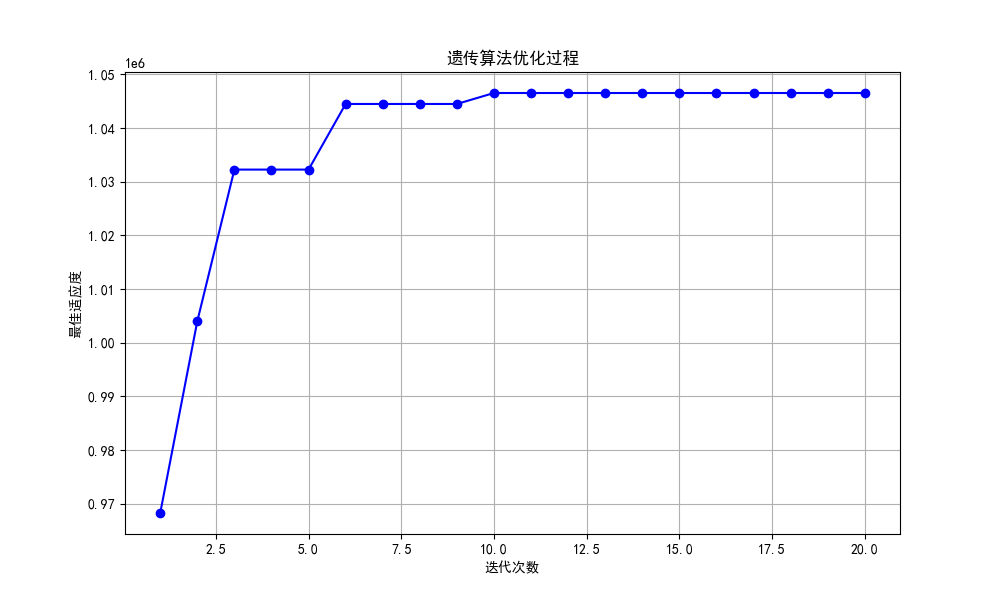
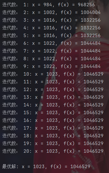
虽然这里得到的就是实际最大值，但由于遗传算法本质上还是一种启发式算法，所以肯定有一定概率找到的是局部最优。

三、蚁群算法（ACO）

蚁群算法最擅长解决的就是诸如上面提到过的TSP问题的组合优化问题。

1.基本概念

首先需要介绍一下蚂蚁找食物的过程。对于每只蚂蚁，在搜索的过程中会在走过的地方留下信息素。在寻路的时候，蚂蚁都会倾向于走信息素浓度高的方向。最核心的是，在蚂蚁寻找食物的过程中，对于距离更短的路径，蚂蚁往返的时间更小，那么往返的次数就会增多，所以信息素的浓度就会更高。所以这条路径就会吸引更多的蚂蚁，循环往复就会成为最优路径。还有，需要注意，信息素会随着时间推移发生挥发，从而防止蚂蚁重复选择较差的路径。

那么在求解问题的过程中，每条边上都会有一个信息素浓度，表示从节点i到节点j的路径上的信息素浓度。之后，为了加快收敛速度，这里默认蚂蚁开了上帝视角，直到每条路径的长度。所以，定义启发式信息为路径长度的倒数。之后，每次蚂蚁选择路径的概率由这个启发式信息和信息素浓度两个参数决定。方法就是每次考察当前节点的所有边连接的没去过的节点，选择某条路径的概率为该路径信息素浓度的次方乘以启发式信息的次方，再除以所有可选路径的上式的累加和。这里，和为重要程度因子，数值越大代表越看重这个参数。

在所有蚂蚁都构建出了一条完整的路径后，由于信息素会挥发，所以每次要考察所有的边，下一轮每条边上的信息素浓度为当前浓度乘以，其中为挥发率。而每只蚂蚁又会释放信息素，所以要在原有的基础上增加的信息素浓度就是，其中Q控制信息素释放的强度，Lk为第k只蚂蚁构建出的这条路径的总长度。

2.基本过程

首先，先随机在地图上设置m个蚂蚁，每次完成路径构建后，让蚂蚁返回初始位置。然后按上述方式挥发并释放信息素，准备下一次的迭代。

这里，可以考虑使用精英策略。在每次迭代时，让本次迭代中构建出最优路径的蚂蚁释放更多的信息素。释放的信息素可以让本次的最优蚂蚁再释放一遍，也可以让该蚂蚁释放Q除以历史最优解的长度的信息素。

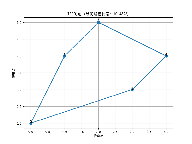
3.练习

import numpy as np
import matplotlib.pyplot as plt
#使用中文字体
from matplotlib.pylab import mpl
mpl.rcParams['font.sans-serif'] = ['SimHei']
mpl.rcParams['axes.unicode_minus'] = False#城市坐标数据
cities = {0: (0, 0),1: (1, 2),2: (3, 1),3: (2, 3),4: (4, 2)
}#计算城市间距离矩阵
def calc_distance_matrix(cities):n = len(cities)dist_matrix = np.zeros((n, n))for i in range(n):for j in range(n):if i != j:x1, y1 = cities[i]x2, y2 = cities[j]dist_matrix[i][j] = np.sqrt((x1 - x2) ** 2 + (y1 - y2) ** 2)return dist_matrix#蚁群算法参数
num_ants = 20  #蚂蚁数量
alpha = 1.0  #信息素重要程度
beta = 2.0  #启发式因子重要程度
rho = 0.5  #信息素挥发率
Q = 100  #信息素强度
num_iterations = 100  #迭代次数#初始化
num_cities = len(cities)
dist_matrix = calc_distance_matrix(cities)  #距离矩阵
pheromone = np.ones((num_cities, num_cities))  #初始信息素矩阵
best_path = None
best_length = float('inf')#主循环
for iteration in range(num_iterations):paths = []  #本代所有蚂蚁的路径lengths = []  #本代所有蚂蚁的路径长度#每只蚂蚁构建路径for ant in range(num_ants):visited = [False] * num_citiespath = []   #该蚂蚁的路径#随机选择起点城市start = np.random.randint(num_cities)path.append(start)visited[start] = True#构建完整路径while len(path) < num_cities:current = path[-1]  #当前位置unvisited = [i for i in range(num_cities) if not visited[i]]#计算选择概率probabilities = []for city in unvisited:pheromone_val = pheromone[current][city]    #信息素浓度heuristic_val = 1 / (dist_matrix[current][city] + 1e-10)  #启发式信息 -> 避免除以零probabilities.append((pheromone_val ** alpha) * (heuristic_val ** beta))#归一化概率total = sum(probabilities)probabilities = [p / total for p in probabilities]#轮盘赌选择下一个城市next_city = np.random.choice(unvisited, p=probabilities)path.append(next_city)visited[next_city] = True#计算路径长度并返回起点length = 0for i in range(num_cities):length += dist_matrix[path[i]][path[(i + 1) % num_cities]]paths.append(path)lengths.append(length)#更新全局最优if length < best_length:best_length = lengthbest_path = path#信息素挥发pheromone *= (1 - rho)#信息素释放for path, length in zip(paths, lengths):for i in range(num_cities):current = path[i]next_city = path[(i + 1) % num_cities]pheromone[current][next_city] += Q / lengthpheromone[next_city][current] = pheromone[current][next_city]  #无向图对称处理#输出结果
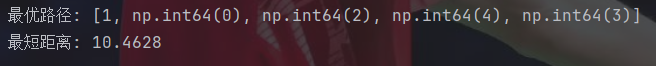
print(f"最优路径: {best_path}")
print(f"最短距离: {best_length:.4f}")#可视化最优路径
x = [cities[i][0] for i in best_path]
y = [cities[i][1] for i in best_path]
x.append(x[0])  #回到起点
y.append(y[0])plt.figure(figsize=(8, 6))
plt.plot(x, y, 'o-', markersize=8, linewidth=2)
plt.title(f'TSP问题 (最优路径长度: {best_length:.4f})')
plt.xlabel('横坐标')
plt.ylabel('纵节点')
for i, (xi, yi) in enumerate(cities.values()):plt.annotate(str(i), (xi, yi), size=12, ha='center')
plt.grid(True)
plt.show()

过程就是模拟着来即可。

四、模拟退火算法（SA）

这也能模拟？！

1.基本概念

首先还是从模拟的自然现象入手。模拟退火算法顾名思义，就是在模拟固体退火的原理。整个过程就是先将金属加热到高温，然后缓慢冷却，让金属从加热前的非晶体状态变成冷却后更稳定的晶体状态。（死去的化学突然开始攻击我）

2.基本过程

整个模拟退火算法是一个双重循环。外循环是退火过程，模拟初始温度很大的情况下，温度逐渐下降的过程。内循环的核心就是Metropolis准则，模拟某一温度下粒子的跳动过程。

在外循环里，会有一个很大的初始温度。除此之外，还会有一个降温系数，越接近1说明降温越慢，一般选择指数降温。此外，还要设置最低温度，控制终止条件。

内循环负责的是在每次温度下，迭代L次，寻找在该温度下能量的最小值，即最优解，并以一定概率接受比当前解更差的解，而这个接受的准则就是Metropolis准则。

这里要先简单说一下爬山算法。假如把一个多峰函数看作一座又一座的山，那么爬山算法的过程就非常暴力，就是每次只往更高的地方走，一旦到达山峰位置，即函数的极大值就停止。那么很明显可以看出，这个算法非常容易陷入局部最优。那么模拟退火算法就是用来改进爬山算法的。在模拟退火算法的内循环中，假如新的解比当前解更优，那么就直接接受即可。而如果新的解比当前解要差，那么和爬山算法不同，模拟退火算法会以一定概率接受这个更差的解。这个概率的计算公式就是：

其中，为新解减去当前解的值，如果小于0就说明新解更优。所以在求最小值时，直接就用目标函数值计算即可。如果是求最大值的话，取个倒数或负数即可。T就是当前的温度。所以，随着温度T的减小，接受概率会逐渐减小，有利于前期扩大搜索范围和后期精确搜索。之后，再生成一个[0,1)的随机数，如果概率P大于这个随机数，那么就接受这个新解。

3.练习

import numpy as np
import math
import random# 目标函数：Rastrigin函数
def rastrigin(x):n = len(x)return 10 * n + sum([(xi ** 2 - 10 * np.cos(2 * math.pi * xi)) for xi in x])# 改进的模拟退火算法（外循环+内循环结构）
def simulated_annealing(objective_func, bounds,max_outer=500, k=100,initial_temp=2000, final_temp=0.01,cooling_rate=0.99):"""参数:objective_func -- 目标函数（最小化）bounds -- 每个变量的取值边界 [(min, max), ...]max_outer -- 外循环最大迭代次数（降温次数）k -- 每个温度下的内循环次数（马尔可夫链长度）initial_temp -- 初始温度final_temp -- 最终温度返回:best_solution -- 最佳解best_value -- 最佳值"""#随机生成初始解current_solution = [random.uniform(b[0], b[1]) for b in bounds]current_value = objective_func(current_solution)#初始化最佳解best_solution = current_solution.copy()best_value = current_value#温度初始化temperature = initial_temp#计算初始扰动范围initial_perturb = [0.1 * (b[1] - b[0]) for b in bounds]#外循环：控制温度下降for outer_iter in range(max_outer):#内循环：在固定温度下进行多次扰动for inner_iter in range(k):#生成新解：在当前解附近随机扰动new_solution = []for j in range(len(bounds)):#计算扰动幅度 -> 随温度降低而减小，但有最小限制min_perturb = 0.001 * (bounds[j][1] - bounds[j][0])  #最小扰动限制max_perturb = initial_perturb[j] * (temperature / initial_temp)perturb_range = max(min_perturb, max_perturb)perturbation = random.uniform(-perturb_range, perturb_range)new_value = current_solution[j] + perturbation#确保新解在边界内new_value = max(bounds[j][0], min(bounds[j][1], new_value))new_solution.append(new_value)#计算新解的目标函数值new_value = objective_func(new_solution)#计算能量差delta = new_value - current_value#如果新解更优，则接受if delta < 0:current_solution = new_solutioncurrent_value = new_value#更新全局最优解if new_value < best_value:best_solution = new_solution.copy()best_value = new_value#如果新解更差，以一定概率接受else:if random.random() < math.exp(-delta / temperature):current_solution = new_solutioncurrent_value = new_value#降低温度temperature *= cooling_rate#每10%进度打印当前状态if outer_iter % (max_outer // 10) == 0:print(f"外循环进度 {outer_iter}/{max_outer}: Temp={temperature:.4f}, Current={current_value:.4f}, Best={best_value:.4f}")#提前终止条件：温度低于最终温度if temperature < final_temp:print(f"提前终止：温度已降至{final_temp}")breakreturn best_solution, best_valueif __name__ == "__main__":#设置搜索边界bounds = [(-10, 10), (-10, 10)]#运行模拟退火算法best_solution, best_value = simulated_annealing(objective_func=rastrigin,bounds=bounds,max_outer=500,  #外循环次数k=100,  #每个温度下的扰动次数initial_temp=2000,final_temp=0.01,  #设置最终温度cooling_rate = 0.99 #设置降温系数)#打印结果print("\n优化结果:")print(f"最佳解: x1={best_solution[0]:.6f}, x2={best_solution[1]:.6f}")print(f"最小值: {best_value:.6f}")

如果不按主外循环和内循环这样写，单纯合并到一个循环的话，搜索效果会非常差。

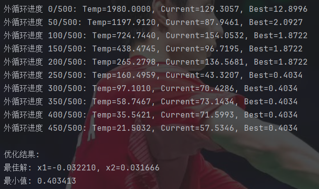
从结果看搜索效果和粒子群差不多。

五、天牛须算法（BAS）

1.基本概念

天牛须算法的优缺点都很明显，优点就是只需要一个个体且运算速度非常快，缺点就是容易陷入局部最优，在处理复杂问题时较为乏力。

天牛须算法就是模拟天牛觅食的过程。天牛在觅食时，会通过两根触角感知到的食物的浓度差异来决定下一步向哪飞行。

2.基本步骤

在求解过程中，首先定义天牛的位置为x，左须的位置为xl，右须的位置为xr，头的朝向随机。之后，在每次迭代时，都随机生成一个向量，接着对这个向量归一化求方向向量d。在有了方向向量后，设置探测距离为，那么左须的位置就是，右须的位置就是。之后，定义步长为step，然后计算两须位置的适应度，哪边更优就向哪边移动步长step。其中，探测距离和步长一般会随着迭代减小，达到前期扩大搜索范围，后期精确搜索。

3.练习

import numpy as np#目标函数定义 -> 五维问题
#求解最小值
def objective_function(x):return (x[0] ** 2 + x[1] ** 2 + 3 * x[2] ** 2 + 4 * x[3] ** 2 + 2 * x[4] ** 2- 3 * x[0] - 4 * x[1] + 5 * x[2] - 2 * x[3] + x[4] + 10)#BAS算法
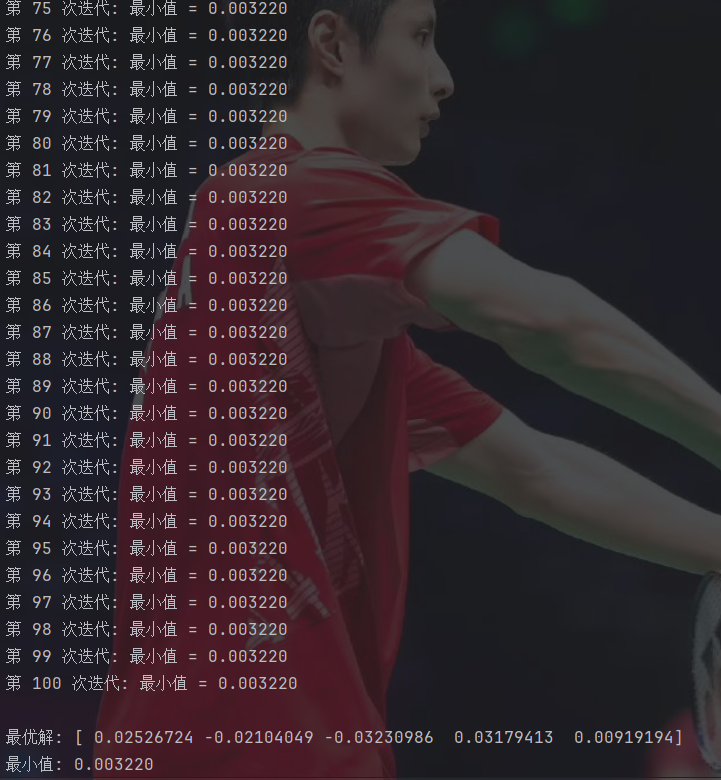
def beetle_antennae_search(dim, bounds, max_iter, step_init, d_init, delta=0.95):"""dim: 变量维度bounds: 变量边界 [min, max]max_iter: 最大迭代次数step_init: 初始移动步长d_init: 初始触须长度delta: 衰减系数"""#随机初始化天牛位置position = np.random.uniform(bounds[0], bounds[1], dim)best_position = position.copy()best_value = objective_function(position)#迭代优化step = step_initd = d_initfor iter in range(max_iter):#生成随机方向向量并归一化direction = np.random.randn(dim)direction /= np.linalg.norm(direction)#计算左右触须位置pos_left = position + d * directionpos_right = position - d * direction#边界约束处理pos_left = np.clip(pos_left, bounds[0], bounds[1])pos_right = np.clip(pos_right, bounds[0], bounds[1])#评估左右位置f_left = objective_function(pos_left)f_right = objective_function(pos_right)#位置更新if f_left < f_right:position = position + step * directionelse:position = position - step * direction#边界约束position = np.clip(position, bounds[0], bounds[1])#更新最优解current_value = objective_function(position)if current_value < best_value:best_value = current_valuebest_position = position.copy()#动态衰减步长和触须长度step *= deltad *= delta#打印进度if iter % 50 == 0:print(f"第 {iter} 次迭代: f={best_value:.6f}")return best_position, best_value#执行
if __name__ == "__main__":#参数设置dim = 5  #变量维度bounds = [-10, 10]  #变量边界max_iter = 200  #迭代次数step_init = 2.0  #初始步长d_init = 3.0  #初始触须长度#运行优化best_solution, best_fitness = beetle_antennae_search(dim, bounds, max_iter, step_init, d_init)#输出结果print("\n===== 优化结果 =====")print(f"最优解: {best_solution}")print(f"最优值: {best_fitness:.6f}")print(f"变量维度: {dim}维, 边界: {bounds}")

这里需要注意边界情况的处理。

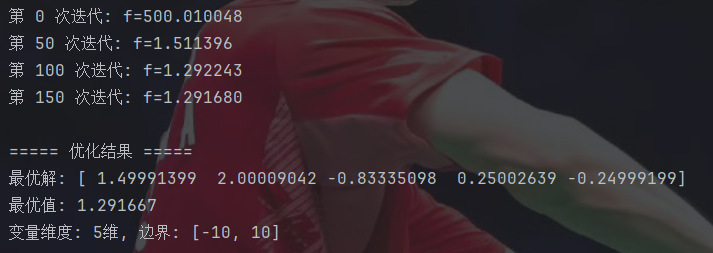
收敛速度是真的快。

六、萤火虫算法（SA）

1.基本概念

萤火虫算法模拟的就是模拟萤火虫通过发光来吸引同伴，亮度越高吸引度越高。

所以，在萤火虫算法中，吸引力与亮度正相关，而亮度和适应度函数相关。此外，还要设置吸引力随距离的增大而指数衰减，即：。其中，表示最大吸引力，一般设置为1。为光吸收速度，控制吸引力的衰减速度。

2.基本步骤

在初始化时，还是随机生成n个萤火虫。之后，还要设置步长因子，，控制随机移动的幅度，一般设置为0.6。在每次迭代时，设置双重循环，计算第i只萤火虫向第j只萤火虫的移动距离，公式为：

在双重循环结束后，就更新最优解并重新计算每只萤火虫的适应度。

3.练习——求解函数最小值

import numpy as np
import matplotlib.pyplot as plt
#使用中文字体
from matplotlib.pylab import mpl
mpl.rcParams['font.sans-serif'] = ['SimHei']
mpl.rcParams['axes.unicode_minus'] = False#Sphere函数
def sphere(x):return np.sum(np.square(x))#萤火虫算法参数
n = 30  #萤火虫数量
d = 5  #问题维度
max_gen = 100  #最大迭代次数
beta0 = 1.0  #初始吸引度
gamma = 0.1  #光吸收系数
alpha = 0.2  #随机步长因子
lb = -5  #搜索下界
ub = 5  #搜索上界#初始化萤火虫种群
fireflies = np.random.uniform(lb, ub, (n, d))
intensity = np.array([sphere(x) for x in fireflies])#记录最优解历史
best_cost_history = []#迭代优化
for gen in range(max_gen):new_fireflies = np.copy(fireflies)for i in range(n):for j in range(n):#如果萤火虫j更亮（即目标函数值更小）if intensity[j] < intensity[i]:#计算欧氏距离r = np.linalg.norm(fireflies[i] - fireflies[j])#计算吸引度beta = beta0 * np.exp(-gamma * r ** 2)#更新位置rand_vec = np.random.uniform(-0.5, 0.5, d)new_fireflies[i] += beta * (fireflies[j] - fireflies[i])new_fireflies[i] += alpha * rand_vec#确保在搜索范围内new_fireflies[i] = np.clip(new_fireflies[i], lb, ub)#更新位置和亮度fireflies = np.copy(new_fireflies)intensity = np.array([sphere(x) for x in fireflies])#记录全局最优best_idx = np.argmin(intensity)best_cost = intensity[best_idx]best_solution = fireflies[best_idx]best_cost_history.append(best_cost)#打印当前最优print(f"第 {gen + 1} 次迭代: 最小值 = {best_cost:.6f}")# 输出最终结果
print(f"\n最优解: {best_solution}")
print(f"最小值: {best_cost:.6f}")# 绘制收敛曲线
plt.figure(figsize=(10, 6))
plt.plot(best_cost_history, 'b-', linewidth=2)
plt.xlabel('迭代次数')
plt.ylabel('最小值')
plt.title('收敛曲线')
plt.grid(True)
plt.show()

这里直接省略了减0.5的步骤，直接生成的-0.5到0.5范围的随机数。

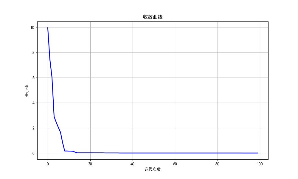
收敛速度还是很快的。

4.练习——聚类

由于萤火虫算法的特点，该算法还可以用来解决聚类问题。过程就是每个萤火虫代表簇中心，将聚类问题中的簇内距离和作为目标函数，求解其最小值。

import numpy as np
import matplotlib.pyplot as plt
#使用中文字体
from matplotlib.pylab import mpl
mpl.rcParams['font.sans-serif'] = ['SimHei']
mpl.rcParams['axes.unicode_minus'] = False
#生成合成数据集
from sklearn.datasets import make_blobs
#层次聚类
from sklearn.cluster import AgglomerativeClustering
#评价聚类结果
from sklearn.metrics import silhouette_score
import time#生成合成数据集
np.random.seed(42)
X, y_true = make_blobs(n_samples=300, centers=4, cluster_std=0.8, random_state=42)#绘制原始数据
plt.figure(figsize=(15, 12))
plt.subplot(2, 2, 1)
plt.scatter(X[:, 0], X[:, 1], c=y_true, cmap='viridis', s=50, edgecolor='k')
plt.title("原始数据")
plt.xlabel("特征1")
plt.ylabel("特征2")#萤火虫聚类算法
class FireflyClustering:def __init__(self, n_clusters=3, n_fireflies=20, max_iter=100,alpha=0.2, beta=1.0, gamma=0.1):self.n_clusters = n_clustersself.n_fireflies = n_firefliesself.max_iter = max_iterself.alpha = alphaself.beta = betaself.gamma = gammaself.centroids = Noneself.labels = Noneself.cost_history = []def _initialize_fireflies(self, X):#随机初始化萤火虫位置（聚类中心）n_features = X.shape[1]fireflies = np.zeros((self.n_fireflies, self.n_clusters * n_features))#每个萤火虫代表一组聚类中心for i in range(self.n_fireflies):#随机选择数据点作为初始中心idx = np.random.choice(X.shape[0], self.n_clusters, replace=False)fireflies[i] = X[idx].flatten()return firefliesdef _calculate_cost(self, X, firefly):#将萤火虫位置重塑为聚类中心centroids = firefly.reshape(self.n_clusters, -1)#计算每个点到最近中心的距离distances = np.zeros((X.shape[0], self.n_clusters))for k in range(self.n_clusters):distances[:, k] = np.linalg.norm(X - centroids[k], axis=1)#分配标签（最近中心）labels = np.argmin(distances, axis=1)#计算目标函数（簇内距离和）cost = 0for k in range(self.n_clusters):cluster_points = X[labels == k]if len(cluster_points) > 0:cost += np.sum(np.linalg.norm(cluster_points - centroids[k], axis=1))return cost, labels, centroidsdef fit(self, X):start_time = time.time()n_features = X.shape[1]fireflies = self._initialize_fireflies(X)intensity = np.zeros(self.n_fireflies)#计算初始强度（成本）for i in range(self.n_fireflies):intensity[i], _, _ = self._calculate_cost(X, fireflies[i])#记录最佳萤火虫best_idx = np.argmin(intensity)best_cost = intensity[best_idx]best_firefly = fireflies[best_idx].copy()self.cost_history.append(best_cost)#萤火虫算法迭代for _ in range(self.max_iter):new_fireflies = fireflies.copy()for i in range(self.n_fireflies):for j in range(self.n_fireflies):#如果萤火虫j比i更亮（成本更低）if intensity[j] < intensity[i]:#计算距离r = np.linalg.norm(fireflies[i] - fireflies[j])#计算吸引度beta = self.beta * np.exp(-self.gamma * r ** 2)#更新位置rand_vec = np.random.uniform(-0.5, 0.5, fireflies[i].shape)new_fireflies[i] += beta * (fireflies[j] - fireflies[i])new_fireflies[i] += self.alpha * rand_vec#更新萤火虫位置和强度fireflies = new_fireflies.copy()for i in range(self.n_fireflies):intensity[i], _, _ = self._calculate_cost(X, fireflies[i])#更新最佳萤火虫current_best_idx = np.argmin(intensity)current_best_cost = intensity[current_best_idx]if current_best_cost < best_cost:best_cost = current_best_costbest_firefly = fireflies[current_best_idx].copy()self.cost_history.append(best_cost)#保存最佳结果self.cost, self.labels, self.centroids = self._calculate_cost(X, best_firefly)self.runtime = time.time() - start_timereturn self#使用萤火虫算法聚类
n_clusters = 4
fa_cluster = FireflyClustering(n_clusters=n_clusters, n_fireflies=30,max_iter=200, alpha=0.2, beta=1.0, gamma=0.1)
fa_cluster.fit(X)#绘制萤火虫聚类结果
plt.subplot(2, 2, 2)
plt.scatter(X[:, 0], X[:, 1], c=fa_cluster.labels, cmap='viridis', s=50, edgecolor='k')
plt.scatter(fa_cluster.centroids[:, 0], fa_cluster.centroids[:, 1],marker='*', s=300, c='red', edgecolor='k', label='聚类中心')
#轮廓系数 -> 越接近1效果越好，接近-1说明越有可能分配错误
plt.title(f"萤火虫聚类\n(轮廓系数: {silhouette_score(X, fa_cluster.labels):.3f}, 所用时间: {fa_cluster.runtime:.2f}s)")
plt.xlabel("特征1")
plt.ylabel("特征2")
plt.legend()#谱系聚类算法
def hierarchical_clustering(X, n_clusters):start_time = time.time()#使用Agglomerative Clustering（谱系聚类的一种）hc = AgglomerativeClustering(n_clusters=n_clusters, linkage='ward')labels = hc.fit_predict(X)#计算聚类中心centroids = np.zeros((n_clusters, X.shape[1]))for k in range(n_clusters):centroids[k] = np.mean(X[labels == k], axis=0)return labels, centroids, time.time() - start_time#使用谱系聚类
hc_labels, hc_centroids, hc_time = hierarchical_clustering(X, n_clusters)#绘制谱系聚类结果
plt.subplot(2, 2, 3)
plt.scatter(X[:, 0], X[:, 1], c=hc_labels, cmap='viridis', s=50, edgecolor='k')
plt.scatter(hc_centroids[:, 0], hc_centroids[:, 1],marker='*', s=300, c='red', edgecolor='k', label='聚类中心')
plt.title(f"谱系聚类法\n(轮廓系数: {silhouette_score(X, hc_labels):.3f}, 所用时间: {hc_time:.2f}s)")
plt.xlabel("特征1")
plt.ylabel("特征2")
plt.legend()#绘制萤火虫算法收敛曲线
plt.subplot(2, 2, 4)
plt.plot(fa_cluster.cost_history, 'b-', linewidth=2)
plt.xlabel('迭代次数')
plt.ylabel('最小簇内距离和')
plt.title('萤火虫算法收敛曲线')
plt.grid(True)plt.tight_layout()
plt.show()#计算簇内距离和（WCSS）
#值越小效果越好
def calculate_wcss(X, labels, centroids):wcss = 0for k in range(len(centroids)):cluster_points = X[labels == k]if len(cluster_points) > 0:wcss += np.sum(np.linalg.norm(cluster_points - centroids[k], axis=1) ** 2)return wcssfa_wcss = calculate_wcss(X, fa_cluster.labels, fa_cluster.centroids)
hc_wcss = calculate_wcss(X, hc_labels, hc_centroids)print(f"\n萤火虫算法的WCSS: {fa_wcss:.2f}")
print(f"谱系聚类法的WCSS: {hc_wcss:.2f}")

这里引入了轮廓系数和簇内距离和的概念，两者都是评价聚类效果的指标。轮廓系数综合考虑了簇内的紧密度和簇间的分离度，取值在[-1,1]上，越靠近1说明效果越好，越靠近-1说明越有可能被分错类了。而簇内距离和只衡量簇内紧密程度，值越接近0效果越好。

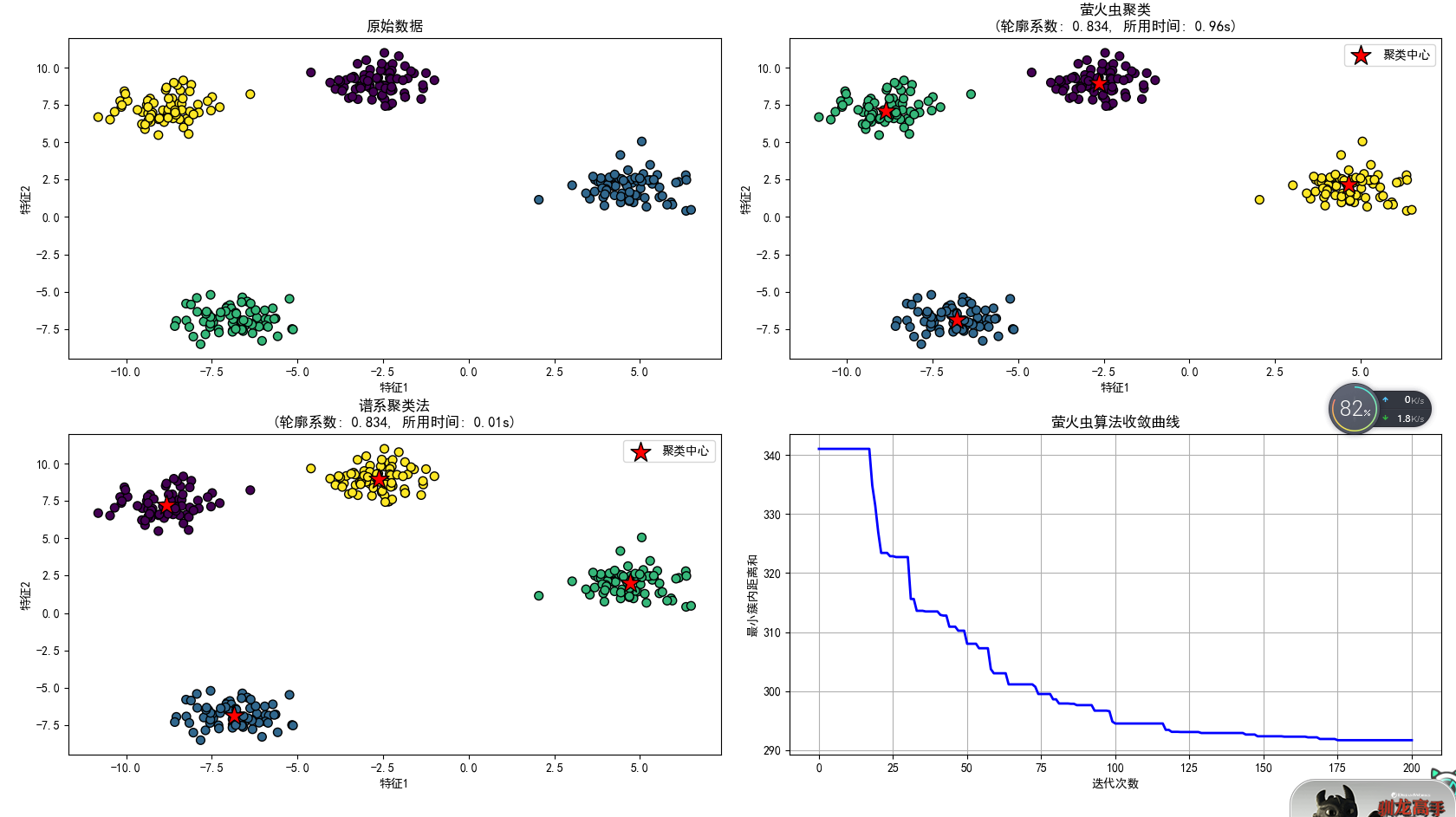
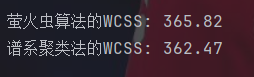
能看出来谱系聚类法不管是效果还是性能都是更强的，但萤火虫算法更适合处理噪声大的数据。

七、鲸鱼优化算法（WOA）

1.基本概念

鲸鱼优化算法模拟的是鲸鱼捕食的过程。首先，在鲸鱼会识别猎物的位置后，会在猎物下方环绕游动，同时螺旋式向上吐出气泡。这些气泡会形成一张圆柱形的网，将猎物困在其中并驱赶到一个更小的区域。最后，鲸鱼会向上冲刺，捕食这些猎物。

鲸鱼优化算法包括三个核心行为，分别是包围猎物，气泡网攻击和随机搜索。

在包围猎物的过程中，每条鲸鱼都会向当前最优解的位置移动，即：

其中，A和C为系数向量，控制包围的强度和方向。

其中，r1和r2均为[0,1]的随机数，a随迭代的加深线性递减。

在气泡网攻击行为中，每次以p的概率选择是否执行螺旋更新。

其中，b为对数螺旋形状的常数，一般设置为1。l为一个在[-1,1]内的常数，负数表示鲸鱼从最优位置向外螺旋探索一点，正数表示向内螺旋开发。

随机探索行为就很好理解了，就是该鲸鱼随机选择另一条鲸鱼并向其移动。

2.基本步骤

首先，还是随机生成n条鲸鱼。之后在每次迭代时，先计算参数a，A和C，其中a的公式为：

之后遍历每条鲸鱼，生成随机数p和l。如果p小于0.5的话，如果A的绝对值小于1，那么就执行包围猎物行为，否则就执行随机搜索行为，如果p大于等于0.5的话，就执行气泡网攻击行为。

3.练习

import numpy as np
import matplotlib.pyplot as plt
#使用中文字体
from matplotlib.pylab import mpl
mpl.rcParams['font.sans-serif'] = ['SimHei']
mpl.rcParams['axes.unicode_minus'] = False#定义Rastrigin函数
def rastrigin(x):A = 10n = len(x)return A * n + sum([(xi ** 2 - A * np.cos(2 * np.pi * xi)) for xi in x])#鲸鱼优化算法
def whale_optimization_algorithm(obj_func, lb, ub, dim, search_agents=10, max_iter=100):"""obj_func : 目标函数lb : 变量下界 (list或标量)ub : 变量上界 (list或标量)dim : 变量维度search_agents : 鲸鱼数量max_iter : 最大迭代次数"""#初始化位置矩阵positions = np.zeros((search_agents, dim))for i in range(dim):if isinstance(lb, list) and isinstance(ub, list):positions[:, i] = np.random.uniform(lb[i], ub[i], search_agents)else:positions[:, i] = np.random.uniform(lb, ub, search_agents)#初始化最优解leader_score = float('inf')leader_pos = np.zeros(dim)#记录收敛过程convergence = np.zeros(max_iter)#主循环for t in range(max_iter):#参数a从2线性减小到0a = 2 - t * (2 / max_iter)for i in range(search_agents):#边界处理positions[i, :] = np.clip(positions[i, :], lb, ub)#计算适应度fitness = obj_func(positions[i, :])#更新领导者if fitness < leader_score:leader_score = fitnessleader_pos = positions[i, :].copy()#更新所有鲸鱼位置for i in range(search_agents):p = np.random.random()if p < 0.5:  #包围猎物或随机搜索r1, r2 = np.random.random(2)A = 2 * a * r1 - aC = 2 * r2if abs(A) < 1:  #包围猎物for j in range(dim):D = abs(C * leader_pos[j] - positions[i, j])positions[i, j] = leader_pos[j] - A * Delse:  #随机搜索rand_idx = np.random.randint(search_agents)for j in range(dim):D = abs(C * positions[rand_idx, j] - positions[i, j])positions[i, j] = positions[rand_idx, j] - A * Delse:  #气泡网攻击b = 1  #螺旋形状常数l = np.random.uniform(-1, 1)for j in range(dim):distance = abs(leader_pos[j] - positions[i, j])positions[i, j] = distance * np.exp(b * l) * np.cos(2 * np.pi * l) + leader_pos[j]#边界处理positions[i] = np.clip(positions[i], lb, ub)convergence[t] = leader_scoreprint(f'第 {t + 1} 次迭代：最小值： {leader_score}')return leader_pos, leader_score, convergence#参数设置
dim = 2  #变量维度
lb = -10  #变量下界
ub = 10  #变量上界
search_agents = 30
max_iter = 50#运行优化算法
best_position, best_value, convergence = whale_optimization_algorithm(rastrigin, lb, ub, dim, search_agents, max_iter
)#输出结果
print("\n优化结果:")
print(f"最优解: {best_position}")
print(f"最小值: {best_value}")#绘制收敛曲线
plt.figure(figsize=(10, 6))
plt.plot(convergence, linewidth=2)
plt.title('收敛曲线')
plt.xlabel('迭代次数')
plt.ylabel('最小值')
plt.grid(True)
plt.show()#可视化搜索空间
x = np.linspace(lb, ub, 100)
y = np.linspace(lb, ub, 100)
X, Y = np.meshgrid(x, y)
Z = np.zeros(X.shape)for i in range(X.shape[0]):for j in range(X.shape[1]):Z[i, j] = rastrigin([X[i, j], Y[i, j]])plt.figure(figsize=(12, 9))
plt.contourf(X, Y, Z, 50, cmap='viridis')
plt.colorbar()
plt.title('Rastrigin函数空间')
plt.xlabel('x1')
plt.ylabel('x2')
plt.scatter(best_position[0], best_position[1], c='red', s=100, marker='*')
plt.show()

注意要先判断p再判断A的绝对值。

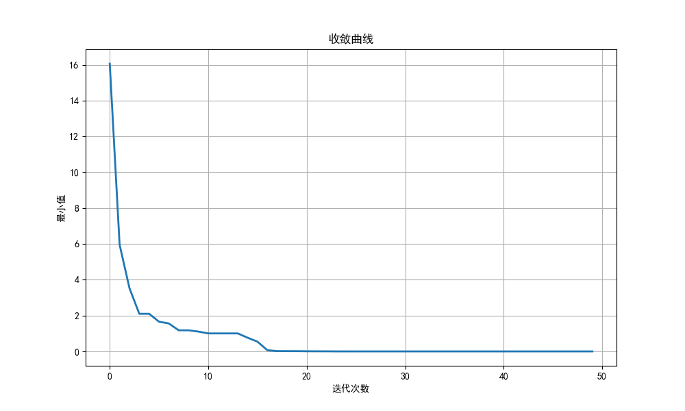
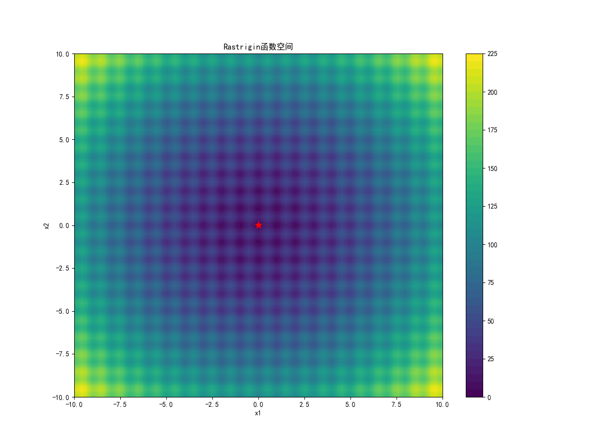
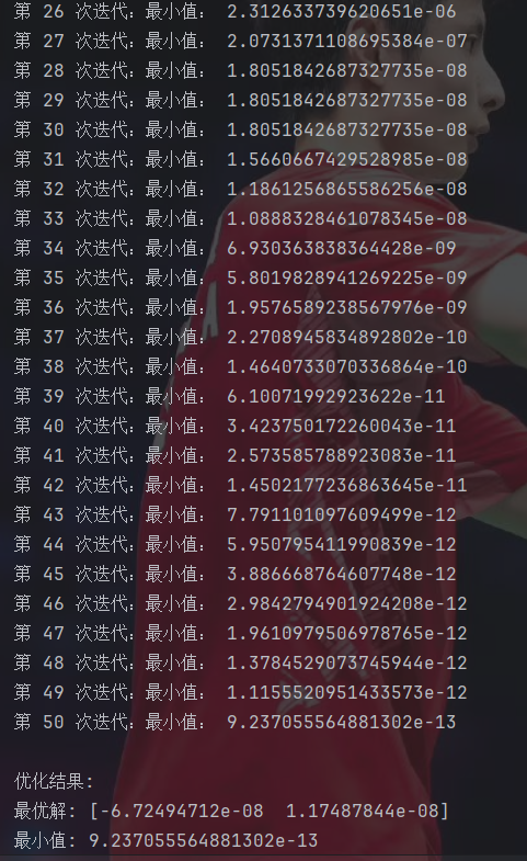
这搜索精度比粒子群算法高太多了……

八、麻雀搜索算法（SSA）

1.基本概念

麻雀搜索算法模拟的就是麻雀在自然界里的行为。麻雀种群分为三种角色，分别是发现者，跟随者和警戒者。发现者负责搜索食物并向同伴传递信息，跟随者负责利用发现者提供的信息进行觅食，警戒者负责警惕环境中的危险。

麻雀搜索算法会将个体划分到这三种角色中，然后各司其职。

发现者因为负责搜索食物的位置，所以通常由适应度好的个体担任。为了模拟现实环境中存在的危险，所以考虑设置一个安全阈值ST，通常取[0.5,1]之间的数。在每次决定怎么移动的时候，随机生成一个[0,1]之间的随机数R2，表示环境中的危险程度。当R2大于等于ST时，位置更新的公式为：

当R2小于ST时，位置更新的公式为：

其中，为(0,1]之间的随机数。Q为一个服从正态分布的随机数。L为一个元素全为1的1×d的单位向量，d为维数。i为迭代次数，maxiter为最大迭代次数。这两个公式就是模拟麻雀分别在环境危险和不危险时的移动策略。

跟随者一般由适应度较差的个体担任，任务是跟随发现者，在发现者找到的较优区域附近进行开发，寻找更好的位置。对于适应度为较差一半的个体，即i>n/2，位置更新的公式为：

而对于其他的个体，位置更新的公式为：

其中，为当前代所有麻雀中的最差位置，为当前代发现者找到的最优位置。A为一个1×d的随机方向矩阵，控制跟随者的移动方向。其中每个元素一半概率为1，一半概率为-1。含义为，对于排名靠后的个体，它们的位置较差，很可能处于饥饿状态，需要飞向其他区域寻找食物，就赋予较大的探索范围。而对于排名靠前的个体，让它们飞向当前最优发现者位置的附近进行开发。

警戒者是在所有个体中随机选择10%~20%的个体担任，负责警戒危险。当警戒者的位置变差，即食物匮乏，或处于边缘，即远离群体中心时，会使整个种群放弃当前位置，随机飞向新的安全区域，从而避免陷入局部最优。如果当前警戒者的适应度不是当前全局最优适应度，那么移动的公式为：

若当前警戒者的适应度是当前全局最优适应度，那公式就为：

其中，为一个服从正态分布的步长参数。和分别为当前个体的适应度和当前最差的适应度。K为[-1,1]范围上的随机数，控制移动方向，为一个很小的常数，避免分母为0。这两个公式的含义为，如果当前警戒者不在最优位置，那么就向当前的最优位置移动。否则，即自己就是当前最优，那么为了避免聚集过密，降低被捕食的风险，就选择向远离种群最差位置的方向移动。

2.基本步骤

首先，初始化随机发现者比例PD，警戒者比例SD和安全阈值ST，一般PD为20%~30%，SD为10%~20%，再随机生成n个麻雀。之后在每次迭代时，先对麻雀根据适应度排序，选择出发现者并更新位置，再让剩下的麻雀为跟随者并更新位置。然后，从整个种群中随机选择出警戒者，重新更新其位置。最后更新全局最优即可。

3.练习

import numpy as np
import matplotlib.pyplot as plt
#使用中文字体
from matplotlib.pylab import mpl
mpl.rcParams['font.sans-serif'] = ['SimHei']
mpl.rcParams['axes.unicode_minus'] = False#定义Rastrigin函数（多峰测试函数）
def rastrigin(x):A = 10return A * len(x) + np.sum([(xi ** 2 - A * np.cos(2 * np.pi * xi)) for xi in x])#麻雀搜索算法参数
n_sparrows = 50  #麻雀数量
dim = 2  #问题维度
max_iter = 100  #最大迭代次数
alpha = 0.1  #衰减系数
PD = 0.2  #发现者比例
SD = 0.1  #警戒者比例
ST = 0.8  #安全阈值
lb = -10  #搜索空间下界
ub = 10  #搜索空间上界#初始化种群
sparrows = np.random.uniform(lb, ub, (n_sparrows, dim))
fitness = np.array([rastrigin(x) for x in sparrows])#记录最佳解
best_index = np.argmin(fitness)
global_best = sparrows[best_index].copy()
global_fitness = fitness[best_index]
best_fitness_history = [global_fitness]#迭代优化
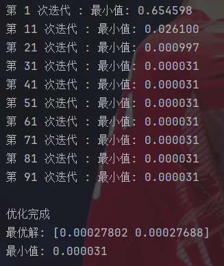
for t in range(max_iter):#排序适应度并选择发现者sorted_indices = np.argsort(fitness)n_discoverers = int(n_sparrows * PD)discoverers = sparrows[sorted_indices[:n_discoverers]]#发现者位置更新R2 = np.random.rand()for i in range(n_discoverers):if R2 < ST:#安全区域：正常搜索Q = np.random.randn()#生成一个符合正态分布的随机数sparrows[sorted_indices[i]] += Q * np.random.randn(dim)else:#危险区域#注意：i_index 是从1开始的排名，不是从0i_index = i + 1decay_factor = np.exp(-i_index / (alpha * max_iter))sparrows[sorted_indices[i]] *= decay_factor#追随者位置更新for i in range(n_discoverers, n_sparrows):#计算当前追随者的排名rank = i - n_discoverers + 1if rank > n_sparrows / 2:#较差追随者Q = np.random.randn()worst_index = sorted_indices[-1]  #最差个体索引worst_position = sparrows[worst_index]current_position = sparrows[sorted_indices[i]]#按维度计算新位置for j in range(dim):sparrows[sorted_indices[i], j] = Q * np.exp((worst_position[j] - current_position[j]) / rank ** 2)else:#普通追随者：飞向最佳发现者best_discoverer = discoverers[0]current_position = sparrows[sorted_indices[i]]#计算 |X - X_best|distance = np.abs(current_position - best_discoverer)#简化计算A_plus_L = np.sign(np.random.rand(dim) - 0.5) * 2  #生成±1的向量sparrows[sorted_indices[i]] = best_discoverer + distance * A_plus_L#警戒者位置更新n_watchers = int(n_sparrows * SD)watcher_indices = np.random.choice(range(n_sparrows), n_watchers, replace=False)#获取最差个体信息worst_index = sorted_indices[-1]worst_position = sparrows[worst_index]worst_fitness = fitness[worst_index]epsilon = 1e-50for idx in watcher_indices:#浮点数相等比较使用容差if abs(fitness[idx] - global_fitness) > 1e-10:#不等于全局最优 -> 飞向全局最优beta = np.random.randn(dim)sparrows[idx] = global_best + beta * np.abs(sparrows[idx] - global_best)else:#等于全局最优 -> 远离最差位置K = np.random.uniform(-1, 1, dim)distance_to_worst = np.abs(sparrows[idx] - worst_position)fitness_diff = fitness[idx] - worst_fitness + epsilon#计算移动步长step = K * distance_to_worst / fitness_diffsparrows[idx] += step#边界处理sparrows = np.clip(sparrows, lb, ub)#更新适应度fitness = np.array([rastrigin(x) for x in sparrows])#更新全局最优current_best_index = np.argmin(fitness)current_best_fitness = fitness[current_best_index]if current_best_fitness < global_fitness:global_best = sparrows[current_best_index].copy()global_fitness = current_best_fitnessbest_fitness_history.append(global_fitness)if t%10==0:print(f"第 {t + 1} 次迭代 : 最小值: {global_fitness:.6f}")#输出结果
print("\n优化完成")
print(f"最优解: {global_best}")
print(f"最小值: {global_fitness:.6f}")#绘制收敛曲线
plt.figure(figsize=(10, 6))
plt.plot(best_fitness_history, 'b-', linewidth=2)
plt.xlabel('迭代次数')
plt.ylabel('最小值')
plt.title('收敛曲线')
plt.grid(True)
plt.show()

这里由于计算起来太复杂了，就采用了简化计算，直接生成+1或-1的向量。

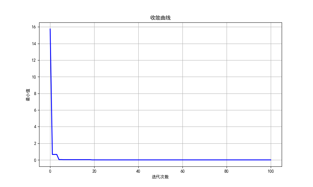
这玩意收敛速度居然这么快……

总结

提高效率，加油！

END