USLR：一款用于脑MRI无偏倚平滑纵向配准的开源工具|文献速递-医学影像算法文献分享

Title

题目

USLR: An open-source tool for unbiased and smooth longitudinal registrationof brain MRI

USLR：一款用于脑MRI无偏倚平滑纵向配准的开源工具

01

文献速递介绍

1. 神经影像学中的许多核心主题，如衰老的影响、疾病进展或治疗效果，本质上都具有纵向性。尽管横断面研究仅能测量群体轨迹，而这类轨迹可能掩盖特定生物标志物的真实演变过程（Nyberg 等，2010），但纵向分析能够揭示真正的个体轨迹，从而减少混杂效应和数据集偏倚，即使在群体平均值与真实效应一致的情况下，也能得出更可靠的估计结果（Maxwell 和 Cole，2007；Kraemer 等，2000）。纵向研究的这种增强效能带来了诸多机遇，包括：（i）更高的敏感性和特异性，可用于检测不同的、部分重叠的萎缩模式（Matuschek 等，2017）；（ii）针对目标效应量减少样本量（Naiji 等，2013）；（iii）为治疗干预提供新的替代终点（Huang 等，2012）。最重要的是，纵向分析产生的个体化测量结果可应用于多种场景，例如治疗后随访或疾病进展监测。   目前存在大量适用于纵向数据分析的统计模型，如重复测量方差分析（ANOVA）、线性混合效应回归或增长模型等（Garcia 和 Marder，2017）。在医学影像领域，向这些统计模型输入适当数据之前，精心设计图像处理流程（如空间标准化或分割）至关重要。然而，大多数最先进的脑图像处理技术是为横断面场景开发的，存在测量可靠性差的问题——这是纵向研究中常见的限制因素（Morey 等，2010；Karch 等，2019）。相反，纵向处理技术能够捕捉时间动态，并利用可用重复测量中的冗余信息，生成更一致、更可靠的结果。例如，受试者特异性模板代表了受试者随时间变化的“平均”解剖结构，可用于脑的纵向分割（Iglesias 等，2016；Cerri 等，2023）。同样，组配准技术可用于更可靠地将图像空间标准化到受试者特异性模板（Joshi 等，2004；Reuter 等，2012）。总之，先采用适当的纵向处理，再结合纵向统计方法（如线性混合效应模型（LME）或重复测量方差分析（ANOVA）），可能会产生更可靠的结果。   尽管如此，纵向处理流程仍需考虑诸多因素。首先是时间点之间不相关的变异源，如信号强度不均匀性、受试者运动以及脑部病变的出现和演变。这些均被视为萎缩估计方法的主要误差来源（Sharma 等，2013）。同样，纵向处理需对随访期间因序列、设备或扫描地点更新导致的信号强度变化具有稳健性，同时也要应对多中心研究中参与者使用不同 MRI 序列、扫描仪、分辨率和场强的情况（Lee 等，2019）。最近的域随机化研究旨在解决多个应用中的这些问题，例如图像超分辨率（Iglesias 等，2023）、分割（Billot 等，2023a）和配准（Hoffmann 等，2022）。此外，不同的偏倚来源，如插值不对称性（即使用特定群体模板或选择某个时间点作为参考图像）或过度的时间正则化，可能会降低方法效能或导致错误结论（Reuter 等，2012；Thompson 等，2011；Yushkevich 等，2010）。    ### 2. 现有的绝大多数经典配准算法基于迭代数值优化，专为成对对齐设计。例如，广泛使用的配准软件包如 NiftyReg（Modat 等，2010）、ANTs（Avants 等，2008）、Elastix（Klein 等，2009）、DARTEL（Ashburner，2007）、FNIRT（Andersson 等，2007）或 IRTK（Schnabel 等，2001）中均实现了此类算法。此外，在深度学习 revolution 中，基于学习的配准方法在有监督（Yang 等，2017；Young 等，2022）和无监督场景（De Vos 等，2019）中均有涌现。同样，这些方法大多基于横断面数据训练。例如，广泛使用的 Voxelmorph 框架可预测密集形变场，用于独立配准成对的 T1 加权图像（Balakrishnan 等，2019）。Hoffmann 等（2022）提出的其扩展版本能够配准任意对比度的成对图像，从而处理扫描仪、序列和协议的差异。已有多种联合线性和非线性基于学习的配准框架被提出，如 DLIR（De Vos 等，2019）或最近的 EasyReg（Iglesias，2023）。   许多纵向研究仅限于 2 个时间点，因此可使用横断面配准流程。例如，在病变随访研究中，基线图像通常被视为参考，因为它通常包含更小的病变（Diez 等，2014；Dufresne 等，2020）。Diez 等（2014）的研究比较了不同的线性和非线性配准方法，以量化多发性硬化（MS）病变的演变。类似地，Dufresne 等（2020）提出了一种用于 MS 配准和变化检测的联合模型。在放射治疗领域，治疗后图像通常配准到治疗前图像以进行治疗随访（Lee 等，2021，2023）。最近，在脑肿瘤切除领域（Baheti 等，2021），多种基于学习的方法被提出，这些方法在训练期间的损失函数中强调逆一致性（Wodzinski 等，2022；Mok 和 Chung，2022b），并处理图像间的缺失对应关系（Mok 和 Chung，2022a）。在此类研究中，基线图像和随访图像可交替作为参考。值得注意的是，现有的纵向配准流程（时间点 > 2）在某种程度上均存在局限性；例如，FreeSurfer 仅限于使用刚性变换。其他现有方法，如 NiftyReg 和 ANTs，可通过在平均模板计算和向该模板的成对配准之间交替进行，用于组配准。然而，将每个时间点独立配准到模板会导致纵向轨迹不连贯。此类方法的一个例子是 Aubert-Broche 等（2013）提出的迭代方法，其初始化使用标准 ICBM152 模板。    ### 3. 在纵向研究中，基于大形变微分同胚度量映射（LDDMM）的测地线回归方法也得到了探索。Ding 等（2019）提出了一种快速基于学习的模型，以基线图像为参考模板，通过成对配准预测受试者的动量。Bône 等（2018）的研究总结了一种迭代构建受试者平均形状并预测其随时间轨迹的方法。与我们的方法不同，他们在图像强度上定义统计模型，这需要初始化受试者特异性模板。而在我们的研究中，我们直接在图像形变上定义统计模型，避免了初始模板的计算。Hadj-Hamou 等（2016）提出了一项与我们类似的研究，该研究使用静态速度场（SVFs）。他们的方法将基线图像作为受试者特异性模板。此外，他们使用经典的（非基于学习的）配准算法（Lorenzi 等，2013），该算法通常比基于学习的方法计算量更大。与我们的研究不同，他们计算的轨迹位于 MNI 空间而非受试者空间，且未提供时间一致性分割。在 Agier 等（2020）的研究中，作者在多受试者组配准场景中使用了与我们观测图相同的图结构。这种结构非常耗时且耗内存，因为它需要使用缓慢的经典配准算法对所有可用时间点进行成对配准。为减少计算需求，他们通过处理图像关键点来降低图像维度。在我们的框架中，我们借助基于学习的配准算法来应对纵向配准的高计算需求。    ### 4. 本研究的贡献有三方面：   - 首先，我们提出了一种用于 MRI 扫描纵向配准的理论框架，该框架具有明确的时间平滑性，对任何时间点无偏倚，且适用于任意数量的时间点和随访间隔。该方法基于空间变换的李代数参数化。   - 其次，我们应用该框架寻找随时间连续的受试者特异性 MRI 轨迹以及受试者特异性模板。为此，我们描述了两种依次应用的空间变换模型：刚性变换和基于静态速度场的非线性微分同胚。   - 第三，我们利用受试者特异性纵向形变，通过标签融合方法从初始横断面分割结果中计算所有时间点的时间一致性分割。   本文的其余部分组织如下：在第 2 节中，我们描述“无偏倚平滑纵向配准”（USLR）框架，并详细讨论概率模型、使用李代数参数化的优势、推断方法以及用于刚性和非线性配准的算法。在第 3 节中，我们介绍两种基于 USLR 的方法，分别用于计算（i）单一稳定的受试者特异性轨迹和（ii）时间一致性分割。在第 4 节中，我们通过一个群组研究用例验证并展示 USLR 框架的优势。最后，第 5 节总结 USLR 的主要优势，并讨论该研究的局限性和未来方向。

Abatract

摘要

We present the ‘‘Unbiased and Smooth Longitudinal Registration’’ (USLR) method, a computational frameworkfor longitudinal registration of brain MRI scans to estimate non-linear image trajectories that are smooth acrosstime, unbiased to any timepoint, and robust to imaging artefacts. It operates on the Lie algebra parameterisationof spatial transforms (which is compatible with rigid transforms and stationary velocity fields for non-lineardeformation) and takes advantage of log-domain properties to solve the problem using Bayesian inference.USRL estimates spatial transformations that: (i) bring all timepoints to an unbiased subject-specific space; and(ii) compute a smooth trajectory across the imaging time-series. We capitalise on learning-based registrationalgorithms and closed-form expressions for fast inference. An Alzheimer’s disease study is used to showcase thebenefits of the pipeline in multiple fronts, such as time-consistent image segmentation to reduce intra-subjectvariability, subject-specific prediction or population analysis using tensor-based morphometry. We demonstratethat such an approach improves upon cross-sectional methods in identifying group differences, which can behelpful in detecting more subtle atrophy levels or in reducing sample sizes in clinical trials.

我们提出了“无偏倚平滑纵向配准”（USLR）方法，这是一种用于脑MRI扫描纵向配准的计算框架，旨在估计具有以下特性的非线性图像轨迹：跨时间平滑、对任何时间点无偏倚，且对成像伪影具有稳健性。该方法基于空间变换的李代数参数化（兼容刚性变换和用于非线性形变的静态速度场），并利用对数域特性通过贝叶斯推断解决问题。   USLR估计的空间变换能够：（i）将所有时间点映射至无偏倚的受试者特异性空间；（ii）计算成像时间序列中的平滑轨迹。我们借助基于学习的配准算法和闭合形式表达式实现快速推断。通过一项阿尔茨海默病研究，从多个层面展示了该流程的优势，例如时间一致性图像分割可降低受试者内变异性、基于受试者特异性的预测，或利用张量形态计量学进行群体分析。我们证明，这种方法在识别组间差异方面优于横断面方法，这有助于检测更细微的萎缩程度或减少临床试验中的样本量。

Conclusion

结论

In this work, we introduce the USLR methodology, a framework forlongitudinal registration of brain MRI scans. It capitalises on Bayesianinference and Lie algebra parameterisations of the spatial transformsto find unobserved deformation fields from each timepoint to a latent,unbiased subject-specific template. We define a probabilistic model inthe space of deformations with pairwise registrations observed ({𝑘 }),and template to timepoint deformations hidden ({𝑛 }). This approachleads to a tractable, fast, and accurate framework that is independentof the registration algorithm (assuming that the deformation fieldcan be parameterised in the log-domain). We could have modelledeach 𝑝({𝑘 }|{𝑇**𝑛 }, 𝜃**𝑘 ) with 𝜃**𝑘 depending on the time distance betweentimepoints. This would, however, require a dedicated penalty functionthat relies on heuristics, as in Ashburner and Ridgway (2013), and theoptimal regularisation will depend on the ultimate goal of the study.As discussed by Ashburner and Ridgway (2013), if the aim is to detectbrain changes (as we do), less regularisation is preferred to reduceestimation bias at the expense of increased noise, because the result isnon-linearly averaged over multiple registrations. Seemingly, it wouldbe also possible to consider {𝑘 } as random variables conditionedto the original images, such that the uncertainties in the registrationpropagate to the estimates of {𝑛 }. However, modelling the posteriordistribution 𝑝({𝑘 }|{𝐼**𝑛 }) (e.g., via sampling) is often difficult and slowdue to the high number of dimensions and strongly non-convex natureof the problem.Importantly, USLR framework generalises to a variety of transformation models; here we use a rigid transform (USLR-rig), to account forglobal misalignment, followed by a non-linear stationary velocity fieldsthat model local geometric differences between timepoints (USLR-diff).In both cases, the use of learning-based algorithms that are robust toacquisition differences (e.g., scanners, sequences, contrasts and resolutions) and that provide fast inferences makes the overall pipelinesuitable for large scale datasets. This is a direct consequence of usingSynthSeg to initialise the rigid registration part (Billot et al., 2023a)and SynthMorph (Hoffmann et al., 2022) as diffeormorphic registrationalgorithm. Furthermore, we have shown its benefits on a case-controlstudy as compared to using cross-sectional processing pipelines.Compared with existing similar approaches in the literature, weare able to compute unbiased and smooth time-varying longitudinaltrajectories. For example, the authors in Joshi et al. (2004) focusedonly on the unbiasedness of the subject-specific template while theauthors of Hadj-Hamou et al. (2016) focused only on computing asingle stationary longitudinal trajectory with the baseline timepointas reference. USLR computes a time-varying trajectory defined on anunbiased template while also outputs a single stationary trajectoryuseful in applications such as linear interpolation and extrapolationacross time or DBM analyses. Moreover, the USLR pipeline outputis successfully applied in downstream tasks and we have shown itsbenefits on a case-control study as compared to using cross-sectionalprocessing pipelines.One limitation of this work is the approximation of the compositionof non-linear deformation fields by the summation of SVFs. As exploredin the supplementary material (Section 3), the error incurred remainedunnoticeable for the age and time span studied in this work, whichis similar to typical follow up times present in clinical trials andobservational studies in elderly adults. However, in contexts with largemorphological changes with time, such as in brain development or postsurgery follow-up, the carried error by the BCH approximation maynot hold and should be assessed, e.g., by visual inspection of the scansdeformed with the fitted transformations.We believe that this work serves as a proof-of-concept and that itopens up the use of USLR in multiple applications as well as extendUSLR to integrate others. For example, we could easily include other Liegroups such as affine transforms (Li et al., 2023; Peter et al., 2018). Or,similarly to Cerri et al. (2023), we could accommodate segmentationmaps in the USLR graph for a joint longitudinal Bayesian registrationand segmentation method. As future directions, the USLR frameworkcan be adapted to contexts with large follow-up changes by writing theobjective function as the composition of deformation fields (rather thanSVFs), and optimise them directly with numerical optimisation. Thisis however computationally much more expensive than the proposedsolution. Finally, we plan to wrap the framework together with someother processing steps (inhomogeneity correction, segmentation, ornormalisation to a template) and publish a comprehensive, well testedopen-source pipeline available to the community.

研究内容总结：   在本研究中，我们提出了USLR（无偏倚平滑纵向配准）方法，这是一种用于脑MRI扫描纵向配准的框架。该框架利用贝叶斯推断和空间变换的李代数参数化，从每个时间点到潜在的、无偏倚的受试者特异性模板中估计未观测的形变场。我们在形变空间中定义了一个概率模型，其中成对配准结果（{𝑘}）为观测值，而模板到时间点的形变（{𝑛}）为隐藏变量。这种方法形成了一个易于处理、快速且准确的框架，且不依赖于特定的配准算法（前提是形变场可在对数域中参数化）。   理论上，我们可以为每个𝑝({𝑘}|{𝑇**𝑛}, 𝜃**𝑘})建模，使𝜃**𝑘依赖于时间点之间的时间距离。但这需要如Ashburner和Ridgway（2013）所述的基于启发式的专用惩罚函数，且最优正则化程度取决于研究的最终目标。正如他们所讨论的，若研究目的是检测脑结构变化（如本研究），应优先选择较少的正则化以减少估计偏倚，尽管这会增加噪声——因为结果是通过多次配准的非线性平均得到的。此外，理论上也可将{𝑘}视为以原始图像为条件的随机变量，使配准中的不确定性传播到{𝑛}的估计中。然而，由于问题的高维度和强非凸性，建模后验分布𝑝({𝑘}|{𝐼**𝑛})（例如通过抽样）通常困难且耗时。    ### USLR框架的核心特性与优势：   USLR框架可推广到多种变换模型。本研究中，我们首先使用刚性变换（USLR-rig）解决全局错位问题，随后通过非线性静态速度场（USLR-diff）建模时间点之间的局部几何差异。在这两种变换中，基于学习的算法对采集差异（如扫描仪、序列、对比度和分辨率）具有稳健性，且能快速推断，使整个流程适用于大规模数据集。这得益于使用SynthSeg初始化刚性配准部分（Billot等，2023a），以及将SynthMorph（Hoffmann等，2022）作为微分同胚配准算法。此外，通过病例对照研究，我们已证明该框架相比横断面处理流程的优势。   与文献中现有类似方法相比，USLR能够计算无偏倚且平滑的时变纵向轨迹。例如，Joshi等（2004）仅关注受试者特异性模板的无偏倚性，而Hadj-Hamou等（2016）仅以基线时间点为参考计算单一稳定的纵向轨迹。USLR则在无偏倚模板上定义时变轨迹，同时输出单一稳定轨迹，适用于时间上的线性插值、外推或基于张量的形态计量学（DBM）分析等场景。此外，USLR的输出已成功应用于下游任务，且在病例对照研究中展现了相比横断面处理流程的优势。    ### 局限性与未来方向：   本研究的一个局限性是通过静态速度场（SVFs）的求和近似非线性形变场的复合。如补充材料（第3节）所示，在本研究涉及的年龄和时间跨度内（与老年人群临床试验和观察性研究中的典型随访时间相似），由此产生的误差并不明显。然而，在随时间发生显著形态变化的场景中（如脑发育或术后随访），BCH近似带来的误差可能不再适用，需通过视觉检查经拟合变换形变后的扫描图像等方式进行评估。   我们认为本研究为概念验证，且为USLR在多领域的应用及扩展奠定了基础。例如，可轻松纳入仿射变换等其他李群（Li等，2023；Peter等，2018）；或借鉴Cerri等（2023）的思路，在USLR图中整合分割图，构建联合纵向贝叶斯配准与分割方法。未来方向包括：通过将目标函数定义为形变场的复合（而非SVFs的求和），并直接通过数值优化求解，使USLR框架适应随访期间变化较大的场景（尽管这会显著增加计算成本）；最终计划将该框架与其他处理步骤（如不均匀性校正、分割或模板标准化）整合，发布一套全面且经过充分测试的开源流程，供学术界使用。

Results

结果

We use the Minimal Interval Resonance Imaging in Alzheimer’sDisease (MIRIAD) dataset (Malone et al., 2013) to exhaustively showthe benefits of using the USLR framework for groupwise analysis inlongitudinal settings. The MIRIAD dataset is a structural MRI cohortof 46 Alzheimer’s disease (AD) subjects and 23 elderly healthy ageingadults with multiple available T1w scans collected at different timepoints. Follow up periods per subject range up to two years and sampling points are unevenly spaced from 2 weeks to one year. Moreover,test-retest scans are available at baseline, and 6 and 38 weeks frombaseline. We consider two separate subsets from the MIRIAD study:first, we build a small set using the baseline test and retest images astwo different timepoints; and second, we build a larger set consistingof all available sessions for all subjects excluding the re-test images.We process all subjects through our USLR processing pipeline as wellas through the longitudinal stream of FreeSurfer for comparison with astandard pipeline widely accepted by the community. The Alzheimer’sdisease neuroimaging initiative (ADNI) dataset is used as a large scaleand more heterogeneous dataset. The ADNI (adni.loni.usc.edu) waslaunched in 2003 as a public–private partnership, led by PrincipalInvestigator Michael W. Weiner, MD. The primary goal of ADNI hasbeen to test whether serial magnetic resonance imaging (MRI), positronemission tomography (PET), other biological markers, and clinicaland neuropsychological assessment can be combined to measure theprogression of mild cognitive impairment (MCI) and early Alzheimer’sdisease (AD). We select a subset of 54 healthy control subjects (CN),73 mild cognitive impairment (sMCI) subjects, 64 Alzheimer’s disease(AD) patients and 78 subjects that converted from MCI to AD (cMCI)during the time span of the study. Diagnostic labels are extracted fromthe ADNI cohort. The average number of timepoints per subject is 5.48(±1.75) with follow up periods of 3.5 (±1.67) years.Furthermore, an Alzheimer’s disease patient from our local datasetis used to better illustrate the benefits of subject-specific analyses.Recruited at the age of 87.5, a total of 11 timepoints across 7.5 yearsof follow up with its associated T1w scans are readily available andprocessed through the USLR pipeline.

4.1. 数据   我们使用阿尔茨海默病最小间隔共振成像（MIRIAD）数据集（Malone 等，2013），全面展示 USLR 框架在纵向场景下组分析中的优势。MIRIAD 数据集是一个结构性 MRI 队列，包含 46 名阿尔茨海默病（AD）患者和 23 名老年健康受试者，均有多组不同时间点采集的 T1 加权扫描图像。每位受试者的随访周期最长达 2 年，采样点间隔不均匀（从 2 周到 1 年不等）。此外，基线、基线后 6 周和 38 周均有重复测试扫描数据。我们从 MIRIAD 研究中选取两个独立子集：第一个子集为小型数据集，将基线的测试和重测图像作为两个不同时间点；第二个子集为大型数据集，包含所有受试者的所有可用会话数据（排除重测图像）。我们通过 USLR 处理流程及 FreeSurfer 纵向流程对所有受试者进行处理，以与学术界广泛认可的标准流程进行对比。   阿尔茨海默病神经影像倡议（ADNI）数据集被用作大规模且更具异质性的数据集。ADNI（adni.loni.usc.edu）于 2003 年启动，是一项公私合作项目，由首席研究员 Michael W. Weiner 博士领导。ADNI 的主要目标是验证是否可通过联合串行磁共振成像（MRI）、正电子发射断层扫描（PET）、其他生物标志物以及临床和神经心理学评估，来衡量轻度认知障碍（MCI）和早期阿尔茨海默病（AD）的进展。我们从 ADNI 队列中选取子集，包括 54 名健康对照受试者（CN）、73 名稳定型轻度认知障碍（sMCI）受试者、64 名阿尔茨海默病（AD）患者以及 78 名在研究期间从 MCI 转化为 AD 的受试者（cMCI）。诊断标签均来自 ADNI 队列。每位受试者的平均时间点数为 5.48（±1.75），随访周期为 3.5（±1.67）年。   此外，我们使用本地数据集中的一名阿尔茨海默病患者，更直观地展示受试者特异性分析的优势。该患者入组时年龄为 87.5 岁，随访 7.5 年期间共采集 11 个时间点的 T1 加权扫描数据，所有数据均通过 USLR 流程处理。

Figure

图

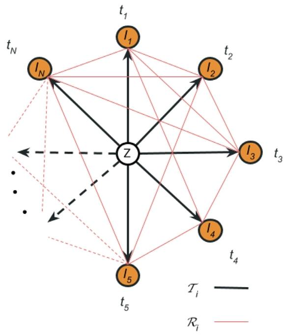
Fig. 1. The graph structure , where all timepoints ‘‘orbit’’ around the unobservedtemplate. In black, our choice of spanning tree of the graph, where all timepointsare connected through the template. The direction of the associated deformation fieldsis from the template to the timepoints, as indicated by the arrows In red, we drawthe observational graph describing the dense pairwise ‘‘noisy’’ registrations of alltimepoints. The direction of this transforms is arbitrary for each subject and knownthroughout the pipeline. The template is depicted at the centre of masses from alltimepoints, ignoring the notion of time between graph nodes. The distance betweentimepoints and the template and between the template themselves is kept equal torepresent the unbiasedness of the method, which treats all timepoints equally

图1 图结构，其中所有时间点围绕未观测模板“环绕”分布。黑色部分为我们选择的图的生成树，所有时间点通过模板相互连接。如箭头所示，相关形变场的方向为从模板指向时间点。红色部分为观测图，描述所有时间点的密集成对“带噪声”配准。对于每个受试者，该变换的方向是任意的，且在整个流程中已知。模板被绘制在所有时间点的质心位置，暂不考虑图节点间的时间概念。时间点与模板之间以及模板自身之间的距离保持相等，以体现该方法的无偏倚性——即对所有时间点一视同仁。

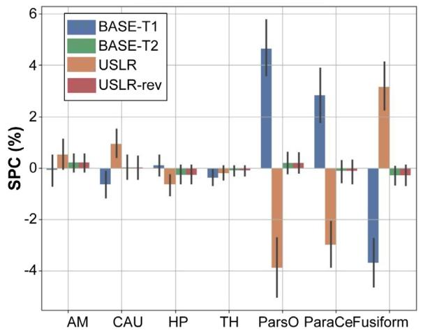
Fig. 2. Symmetrised percent change (SPC) for different cortical and subcorticalbrain regions: amygdala (AM); caudate (CAU); hippocampus (HP); thalamus (TH);pars opercularis (ParsO); paracentral (ParaCe); and fusiform. BASE-T1 (T2) initialisetimepoint 2 (1) with the segmentation of timepoint 1 (2). USLR and USLR-rev processtimepoints in reversed order.

图2 不同皮质及皮质下脑区的对称化百分比变化（SPC）：杏仁核（AM）、尾状核（CAU）、海马（HP）、丘脑（TH）、岛盖部（ParsO）、中央旁小叶（ParaCe）和梭状回。BASE-T1（T2）以时间点1（2）的分割结果初始化时间点2（1）的分割。USLR和USLR-rev以相反顺序处理时间点。

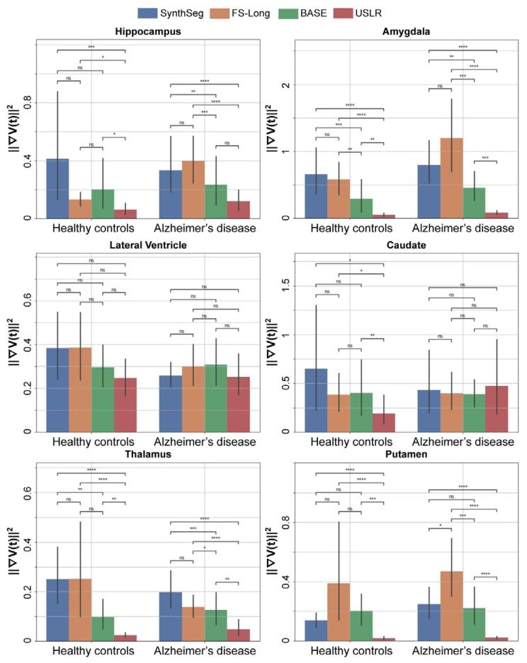
Fig. 3. Evaluating trajectory smoothness using Eq. (18) stratified by diagnosticcategory. We compare four different models: SynthSeg, longitudinal Freesurfer segmentations (FS-Long), longitudinal refinement using the baseline image as template(BASE) and USLR. Significant differences in smoothness are found in a Wilcoxon-ranktest between methods for (*) 1 ⋅ 10−2 < 𝑝 < 5 ⋅ 10−2 , () 1 ⋅ 10−3 < 𝑝 < 1 ⋅ 10−2 , (*)1 ⋅ 10−4 < 𝑝 < 1 ⋅ 10−3 and () 𝑝 < 1 ⋅ 10−4 thresholds

图3 采用公式（18）按诊断类别分层评估轨迹平滑度。我们比较了四种不同模型：SynthSeg、纵向FreeSurfer分割（FS-Long）、以基线图像为模板的纵向优化（BASE）以及USLR。通过Wilcoxon秩检验发现，不同方法间的平滑度存在显著差异，显著性水平标注如下：（）1×10⁻²＜𝑝＜5×10⁻²，（**）1×10⁻³＜𝑝＜1×10⁻²，（**）1×10⁻⁴＜𝑝＜1×10⁻³，（）𝑝＜1×10⁻⁴。

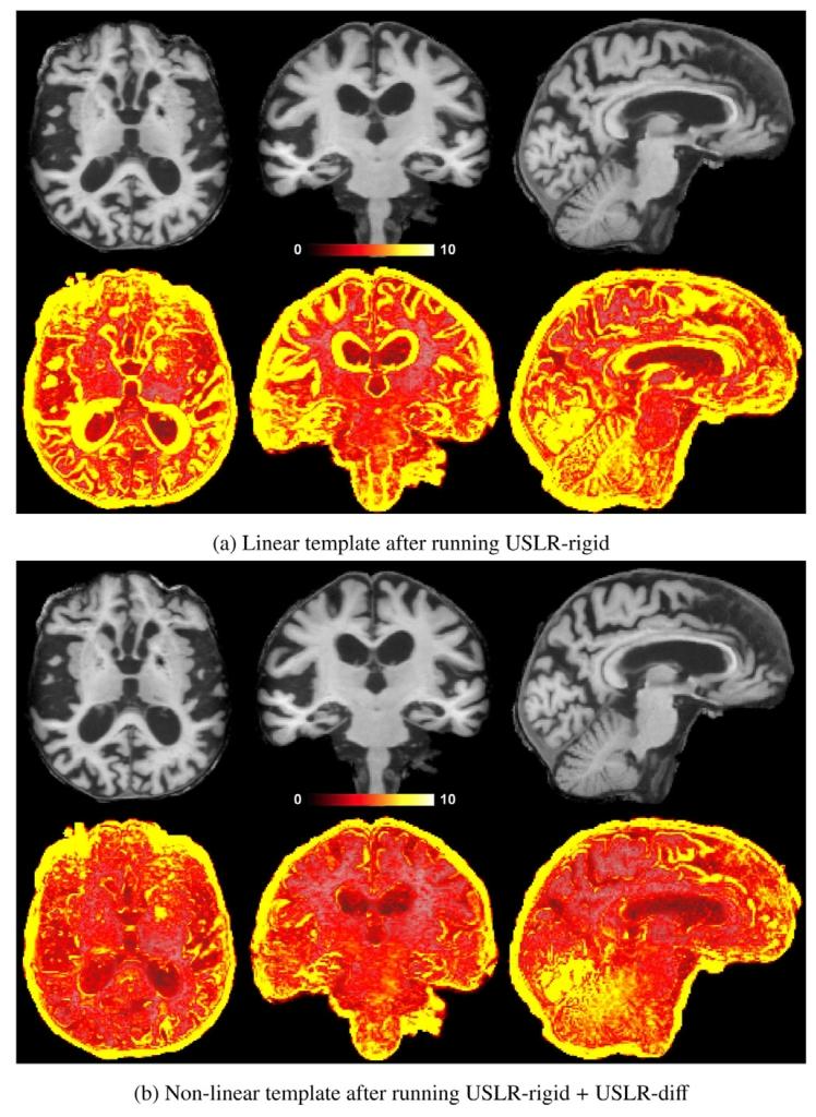
Fig. 4. Example of a template of an Alzheimer’s disease subject followed-up for atotal of 7.5 years with 𝐿 = 11 scans from a local cohort. On the top row, the meanT1w subject-specific template and on the bottom row, the standard deviation of theintensities between all the resampled and normalised timepoints. The larger variance inthe linear template leads to misleading intensity values, such as around the ventricles,where it looks like grey-matter tissue. The non-linear template is sharper and preventsartificial intensity values.

图4 一名阿尔茨海默病受试者的模板示例，该受试者来自本地队列，随访总时长为7.5年，共进行了𝐿=11次扫描。上行图像为受试者特异性T1加权平均模板，下行图像为所有重采样和标准化时间点之间的信号强度标准差。线性模板的较大方差会导致误导性的强度值，例如在脑室周围区域，其表现类似灰质组织。而非线性模板更清晰，可避免出现人工伪影强度值。

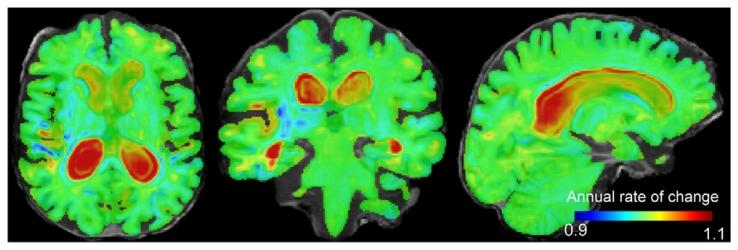
Fig. 5. Jacobian determinant of the 1-year subject-specific estimated trajectory of anAlzheimer’s disease patient overlaid on its non-linear template. Hot colours (> 1)indicate expansion and cold colours (< 1) indicate contraction over time. The valueof each voxel indicates the annual rate of change.

图5 阿尔茨海默病患者1年受试者特异性估计轨迹的雅可比行列式，叠加于其非线性模板之上。暖色（>1）表示随时间扩张，冷色（<1）表示随时间收缩。每个体素的值代表年度变化率。

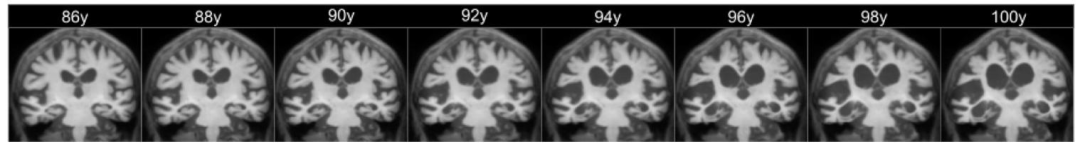
Fig. 6. Subject-specific prediction at the voxel level, computed by deforming the non-linear subject-specific template using the estimated SVF trajectories. The age range shownspans from 1.5 years prior the baseline observation to 5 years after the last observation. The real duration of the study ranges from 87.5 to 95 years old.

图6 体素水平的受试者特异性预测结果，通过使用估计的静态速度场（SVF）轨迹对非线性受试者特异性模板进行形变计算得到。所示年龄范围涵盖基线观测前1.5年至最后一次观测后5年。研究的实际持续时间范围为87.5至95岁。

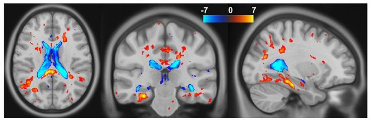
Fig. 7. T-test results on the Jacobian determinants between healthy controls andAlzheimer’s disease subjects, computed using USLR. We show the t-values thresholdedat 𝑝 = 0.05 corrected for multiple comparisons using FDR.

图7 使用USLR计算的健康对照者与阿尔茨海默病受试者之间雅可比行列式的t检验结果。图中展示的t值以𝑝=0.05为阈值（通过虚假发现率（FDR）校正多重比较）。

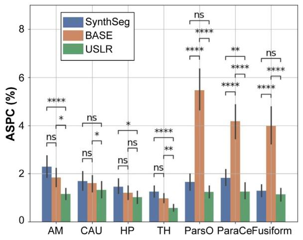
Fig. 8. Absolute symmetrised percent change (ASPC) for different cortical and subcortical brain regions: amygdala (AM); caudate (CAU); hippocampus (HP); thalamus(TH); pars opercularis (ParsO); paracentral (ParaCe); and fusiform. Three segmentationmethods are compared: (i) SynthSeg, which is the original cross-sectional segmentations; (ii) BASE, which is the longitudinal refinement using one acquisition as referencetemplate; and (iii) USLR. A Wilcoxon-rank test is used for statistical significance with(*) 1 ⋅ 10−2 < 𝑝 < 5 ⋅ 10−2 , () 1 ⋅ 10−3 < 𝑝 < 1 ⋅ 10−2 , (*) 1 ⋅ 10−4 < 𝑝 < 1 ⋅ 10−3 and() 𝑝 < 1 ⋅ 10−4 thresholds.

图8 不同皮质及皮质下脑区的绝对对称化百分比变化（ASPC）：杏仁核（AM）、尾状核（CAU）、海马（HP）、丘脑（TH）、岛盖部（ParsO）、中央旁小叶（ParaCe）和梭状回。比较了三种分割方法：（i）SynthSeg，即原始横断面分割；（ii）BASE，即使用一次采集作为参考模板的纵向优化；（iii）USLR。采用Wilcoxon秩检验进行统计显著性分析，显著性水平标注如下：（）1×10⁻²＜𝑝＜5×10⁻²，（**）1×10⁻³＜𝑝＜1×10⁻²，（**）1×10⁻⁴＜𝑝＜1×10⁻³，（）𝑝＜1×10⁻⁴。

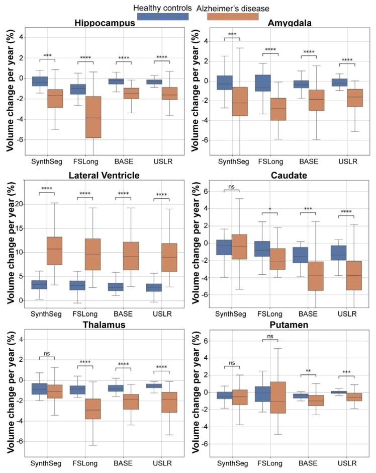
Fig. 9. Sensitivity analysis computing the trajectory’s slope of 6 different ROI volumesper subject. In each figure, we compare three different segmentation methods. From leftto right: cross-sectional SynthSeg, the longitudinal stream of Freesurfer, a longitudinalrefinement using the baseline image as template and our USLR framework. Cognitivelynormal subjects are grouped in blue while AD subjects in dark orange. Significantdifferences in mean slopes are found in a Wilcoxon-rank test between groups for (*)1 ⋅ 10−2 < 𝑝 < 5 ⋅ 10−2 , () 1 ⋅ 10−3 < 𝑝 < 1 ⋅ 10−2 , (*) 1 ⋅ 10−4 < 𝑝 < 1 ⋅ 10−3 and ()𝑝 <* 1 ⋅ 10−4 thresholds.

图9 敏感性分析：计算每位受试者6个不同感兴趣区（ROI）体积的轨迹斜率。每张图中比较了三种不同的分割方法，从左到右依次为：横断面SynthSeg、FreeSurfer纵向流程、以基线图像为模板的纵向优化，以及我们的USLR框架。认知正常受试者以蓝色分组，阿尔茨海默病（AD）受试者以深橙色分组。通过Wilcoxon秩检验发现，组间平均斜率存在显著差异，显著性水平标注如下：（）1×10⁻²＜𝑝＜5×10⁻²，（**）1×10⁻³＜𝑝＜1×10⁻²，（**）1×10⁻⁴＜𝑝＜1×10⁻³，（）𝑝＜1×10⁻⁴。

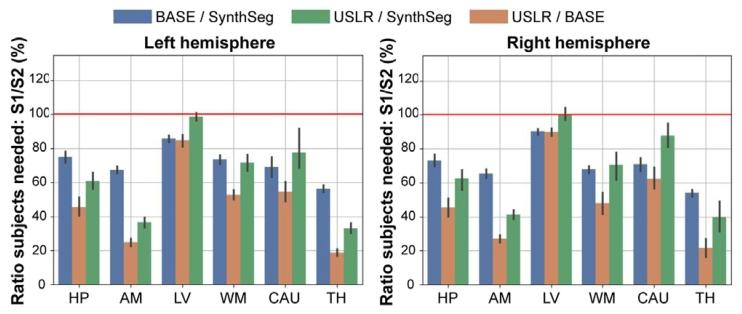
Fig. 10. Power analysis showing the fraction of required subjects comparing segmentation methods S1 and S2. In blue, S1=BASE and S2=SynthSeg; in green S1=USLRand S2=SynthSeg; and in orange, S1=USLR and S2=BASE. A value < 100% indicatesthat S1 needs less subjects than S2 for given study specifications (power, target effectsize, target power, etc.). The red line indicates that the same number of subjects arerequired between S1 and S2. BASE refers to longitudinal processing of timepoints usingthe baseline image as template. In the 𝑥-axis, we show the result of considering differentsubcortical region as primary outcome of the study

图10 效能分析：展示分割方法S1和S2所需受试者比例的对比。蓝色曲线代表S1=BASE与S2=SynthSeg的对比；绿色曲线代表S1=USLR与S2=SynthSeg的对比；橙色曲线代表S1=USLR与S2=BASE的对比。当数值＜100%时，表明在给定研究规格（效能、目标效应量、目标检验效能等）下，S1所需的受试者数量少于S2。红色线表示S1和S2所需的受试者数量相同。BASE指以基线图像为模板对时间点进行的纵向处理。x轴展示将不同皮质下区域作为研究主要结局指标的分析结果。

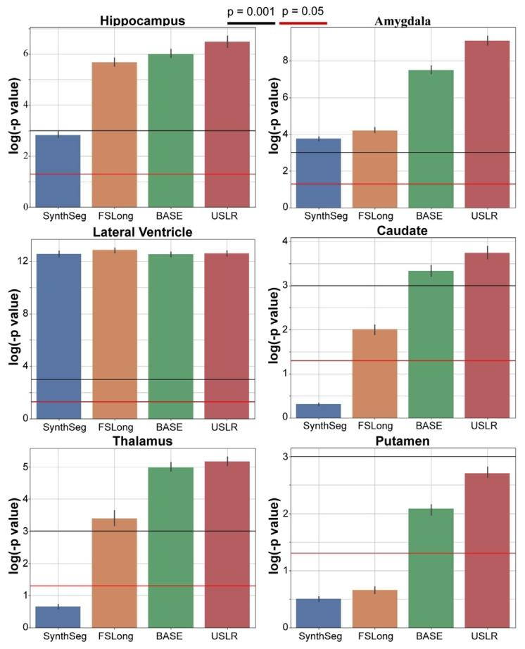
Fig. 11. Linear mixed-effects model with random intercept and slope. We plot the𝑙𝑜𝑔(𝑝* − 𝑣𝑎𝑙𝑢𝑒) of a contrast comparing time evolution between cognitively normalsubjects and AD subjects. The bars represent the median value of 𝑁 = 1000 bootstrapsample. We compare three different segmentation methods: cross-sectional SynthSeg(blue), the longitudinal stream of Freesurfer (dark orange) and our USLR framework(green). Red line represents a 𝑝-value of 5 ⋅ 10−2 and the black line a 𝑝-value of 1 ⋅ 10−3 .

图11 带有随机截距和斜率的线性混合效应模型。图中绘制了对比认知正常受试者与阿尔茨海默病（AD）受试者时间演变差异的𝑙𝑜𝑔(𝑝值)。误差条代表𝑁=1000次bootstrap抽样的中位数。我们比较了三种不同的分割方法：横断面SynthSeg（蓝色）、FreeSurfer纵向流程（深橙色）以及我们的USLR框架（绿色）。红色线代表𝑝值为5×10⁻²，黑色线代表𝑝值为1×10⁻³。

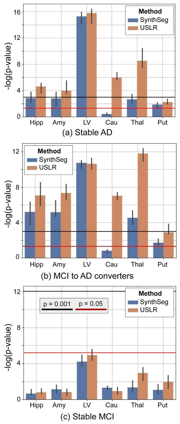
Fig. 12. Linear mixed-effects model with random intercept and slope. The fixed effectsfeatures are time, age, sex, total intracranial volume and the interaction of the interceptand time with diagnosis (stable MCI, MCI to AD converter and stable AD). We plotthe 𝑙𝑜𝑔(𝑝 − 𝑣𝑎𝑙𝑢𝑒) of a contrast comparing time evolution between cognitively normalsubjects and the three diagnostic labels. The bars represent the median value of𝑁* = 1000 bootstrap sample. We compare the USLR framework to SynthSeg. Red linerepresents a 𝑝-value of 5⋅10−2 and the black line a 𝑝-value of 1⋅10−3 . Selected ROIs are:hippocampus (Hipp), amygdala (Amy), lateral ventricle (LV), caudate (Cau), thalamus(Thal) and putamen (Put)

图12 带有随机截距和斜率的线性混合效应模型。固定效应变量包括时间、年龄、性别、总颅内体积，以及截距和时间与诊断结果（稳定型轻度认知障碍（MCI）、从MCI转化为AD的患者、稳定型AD）的交互项。图中绘制了对比认知正常受试者与三种诊断标签受试者时间演变差异的𝑙𝑜𝑔(𝑝值)。误差条代表𝑁=1000次bootstrap抽样的中位数。我们将USLR框架与SynthSeg进行比较。红色线代表𝑝值为5×10⁻²，黑色线代表𝑝值为1×10⁻³。所选感兴趣区（ROIs）包括：海马（Hipp）、杏仁核（Amy）、侧脑室（LV）、尾状核（Cau）、丘脑（Thal）和壳核（Put）。