RoMa: Robust Dense Feature Matching论文精读（逐段解析）

RoMa: Robust Dense Feature Matching论文精读（逐段解析）

Robust Dense Feature Matching（稳健密集特征匹配）

CVPR 2024

Johan Edstedt、Qiyu Sun、Georg Bokman、Marten Wadenback、Michael Felsberg（加粗作者也是DKM的作者，DKM: Dense Kernelized Feature Matching for Geometry Estimation论文精读（逐段解析））

林雪平大学（瑞典）、华东理工大学、查尔姆斯理工大学（瑞典）

Project Page：https://parskatt.github.io/RoMa/

论文地址：https://arxiv.org/pdf/2305.15404

github：https://github.com/Parskatt/RoMa

RoMa 是一种强大的密集特征匹配器，能够估计几乎任何图像对的像素密集扭曲和可靠的结果。

特征匹配的核心目标是在两张拍摄同一3D场景的图像之间建立像素级的对应关系，这是许多高级计算机视觉任务的基础。密集特征匹配方法不同于传统的稀疏方法，它试图为图像中的每个像素都找到对应点，而不仅仅是关键点。这种方法的优势在于能够提供更完整的场景理解，但也面临着更大的计算复杂度和鲁棒性挑战。

作者提出的核心创新在于巧妙地结合了两种不同尺度的特征。DINOv2作为一个大规模预训练的基础模型，其特征具有很强的语义理解能力和泛化性能，但分辨率相对较低，无法提供精确的像素级定位。因此，作者采用"冻结"策略，即保持DINOv2的权重不变，避免过拟合到特定数据集。同时，他们训练了专门的ConvNet来提取细粒度特征，这些特征虽然可能不如DINOv2那样具有强大的语义理解能力，但能够提供精确的空间定位信息。将这两种特征组合成特征金字塔，既保证了匹配的鲁棒性又确保了定位的精度。

在匹配解码阶段，作者采用了transformer架构，但关键创新在于预测锚点概率而不是直接回归坐标。这种设计能够处理匹配过程中的多模态问题，即一个特征点可能对应多个候选匹配点的情况。通过概率分布的形式表达这种不确定性，模型能够更好地处理歧义性匹配场景。损失函数的设计也体现了作者对匹配问题本质的深刻理解：在粗糙匹配阶段使用分类损失来处理多模态分布，在精细化阶段使用鲁棒回归损失来处理相对确定的单模态分布。

============================================================================
【算法总体流程总结】

1、第一阶段：特征提取与融合
使用冻结的DINOv2编码器提取粗糙特征：输入两张图像 $I^A,I^B$，通过冻结的DINOv2编码器提取步长为14的粗糙特征图 ${\phi }_{\mathrm{coarse}}^A,{\phi }_{\mathrm{coarse}}^B$（512维），这些特征具有强大的语义理解能力和跨域泛化性能。
DKM继承的匹配编码器特征融合：将DINOv2特征与高斯过程（GP）匹配编码器 $E_{\theta }$ 的输出进行融合。GP模块处理两张图像的DINOv2特征对，生成512维的匹配特定特征，最终形成1024维的融合特征向量。

2、第二阶段：Transformer匹配解码器处理
使用Transformer匹配解码器处理：融合特征输入到由5个ViT块组成的Transformer解码器（8个注意力头，隐藏维度1024，MLP大小4096），关键创新是不使用位置编码，仅依赖特征相似性传播。
得到4096个分类锚点和额外1维用于可匹配性得分：Transformer输出维度为 $B\times H\times W\times (K+1)$，其中 $K=64\times 64=4096$ 个分类锚点用于匹配预测，额外1维存储可匹配性得分 $p^A(x^A)$，用于判断当前像素是否存在有效匹配。

3、第三阶段：回归分类化处理
锚点概率预测：
- 离散化：将连续坐标空间划分为64×64网格，每个网格点作为一个锚点 $m_k$
- 对每个锚点预测匹配概率：模型预测每个锚点的激活概率 ${\pi }_k(x^A)$，形成条件分布 $p_{\mathrm{coarse},\theta }(x^B|x^A)={\sum }_{k=1}^K{\pi }_k(x^A){\mathcal{B}}_{m_k}$
- 通过局部softargmax恢复亚像素精度：选择最优锚点 $k^{\ast }(x)={\mathrm{argmax}}_k{\pi }_k(x)$，然后在其2×2邻域 $N_4(k^{\ast })$ 内进行概率加权平均
- 解码为扭曲场：${\hat{W}}_{\mathrm{coarse}}^{A\to B}=\frac{{\sum }_{i\in N_4(k^{\ast })}{\pi }_i{m}_i}{{\sum }_{i\in N_4(k^{\ast })}{\pi }_i}$

4、第四阶段：多尺度细化阶段
多尺度细化架构：使用专门的VGG19 ConvNet作为精细特征提取器，与DINOv2特征解耦训练。细化器由4个ConvNet组成，步长分别为 {1,2,4,8}\{1,2,4,8\}{1,2,4,8}，形成从粗到细的金字塔结构。
递归细化过程：从最粗糙尺度（i=3，步长=8）开始，对每个尺度 i∈{3,2,1,0}i \in \{3,2,1,0\}i∈{3,2,1,0}：
- 输入：精细特征 ${\phi }_i^A,{\phi }_i^B$ + 上一尺度扭曲 ${\hat{W}}_{i+1}^{A\to B}$ + 可匹配性 $p_{\theta ,i+1}^A$
- 输出：当前尺度扭曲 ${\hat{W}}_i^{A\to B}$ + 更新可匹配性 $p_{i,\theta }^A$
- 预测残差偏移量和logit偏移量
- 双线性上采样到下一尺度分辨率

最终输出：高分辨率密集扭曲场 ${\hat{W}}^{A\to B}$ 和可匹配性概率 $p^A$，实现像素级的精确匹配。

Abstract

1. Introduction

Feature matching is an important computer vision task that involves estimating correspondences between two images of a 3D scene, and dense methods estimate all such correspondences. The aim is to learn a robust model, i.e., a model able to match under challenging real-world changes. In this work, we propose such a model, leveraging frozen pretrained features from the foundation model DINOv2. Although these features are significantly more robust than local features trained from scratch, they are inherently coarse. We therefore combine them with specialized ConvNet fine features, creating a precisely localizable feature pyramid. To further improve robustness, we propose a tailored transformer match decoder that predicts anchor probabilities, which enables it to express multimodality. Finally, we propose an improved loss formulation through regression-byclassification with subsequent robust regression. We conduct a comprehensive set of experiments that show that our method, RoMa, achieves significant gains, setting a new state-of-the-art. In particular, we achieve a $36\%$ improvement on the extremely challenging WxBS benchmark. Code is provided at github.com/Parskatt/RoMa.

【翻译】特征匹配是计算机视觉中一个重要任务，涉及估计3D场景的两张图像之间的对应关系，密集方法估计所有这样的对应关系。目标是学习一个鲁棒的模型，即能够在具有挑战性的现实世界变化下进行匹配的模型。在这项工作中，我们提出了这样一个模型，利用来自基础模型DINOv2的冻结预训练特征。尽管这些特征比从头训练的局部特征显著更鲁棒，但它们本质上是粗糙的。因此，我们将它们与专门的ConvNet精细特征相结合，创建一个精确可定位的特征金字塔。为了进一步提高鲁棒性，我们提出了一个定制的transformer匹配解码器，预测锚点概率，这使其能够表达多模态性。最后，我们通过回归分类和后续的鲁棒回归提出了一个改进的损失公式。我们进行了一系列全面的实验，表明我们的方法RoMa取得了显著的收益，创造了新的最先进水平。特别是，我们在极具挑战性的WxBS基准上取得了$36\%$的改进。代码可在github.com/Parskatt/RoMa获取。

Figure 1. RoMa is robust, i.e., able to match under extreme changes. We propose RoMa, a model for dense feature matching that is robust to a wide variety of challenging real-world changes in scale, illumination, viewpoint, and texture. We show correspondences estimated by RoMa on the extremely challenging benchmark $\mathbf{WxBS}$ [35], where most previous methods fail, and on which we set a new state-of-the-art with an improvement of $36\%$ mAA. The estimated correspondences are visualized by grid sampling coordinates bilinearly from the other image, using the estimated warp, and multiplying with the estimated confidence.

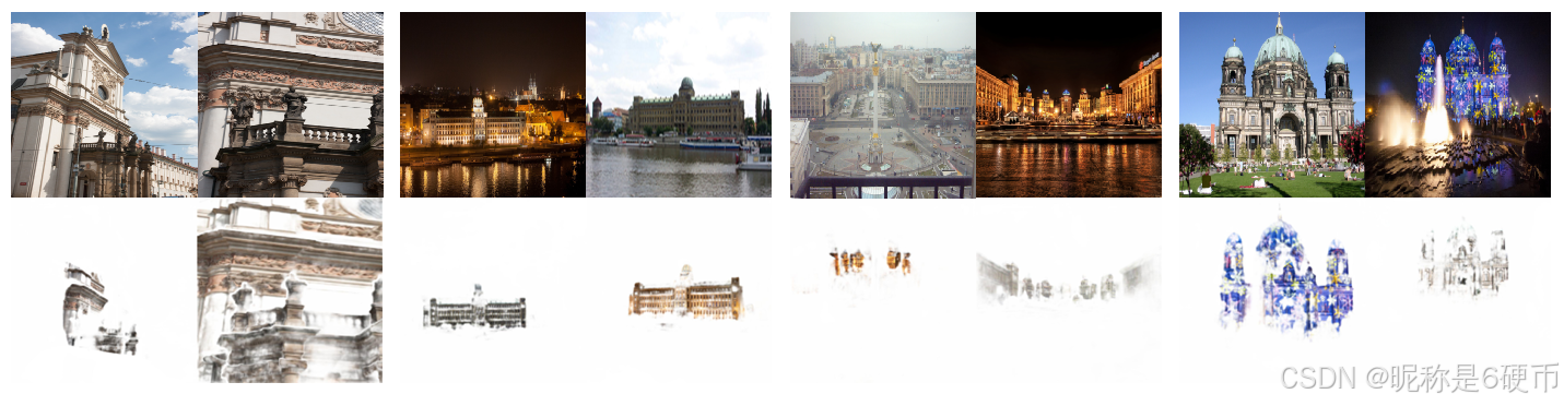
【翻译】图1. RoMa是鲁棒的，即能够在极端变化下进行匹配。我们提出RoMa，一个密集特征匹配模型，对各种具有挑战性的现实世界变化具有鲁棒性，包括尺度、光照、视角和纹理变化。我们展示了RoMa在极具挑战性的基准$\mathbf{WxBS}$ [35]上估计的对应关系，大多数以前的方法在该基准上都失败了，而我们在该基准上创造了新的最先进水平，mAA提高了$36\%$。估计的对应关系通过使用估计的变形从另一图像进行网格采样坐标双线性插值，并乘以估计的置信度来可视化。

【解析】这个图展示了RoMa方法在极端条件下的匹配能力。$\mathbf{WxBS}$基准测试包含了现实世界中最具挑战性的匹配场景，涵盖了大幅度的尺度变化、极端的光照条件、大角度的视角变换以及复杂的纹理变化。传统方法在这些极端条件下往往会失效，因为它们依赖的局部特征描述子容易受到这些变化的影响而变得不稳定。可视化方法采用了网格变形的方式，通过估计的变形场将一张图像的网格坐标映射到另一张图像上，然后用置信度加权，这样能够直观地展示匹配的质量和覆盖范围。

Feature matching is the computer vision task of from two images estimating pixel pairs that correspond to the same 3D point. It is crucial for downstream tasks such as 3D reconstruction [43] and visual localization [40]. Dense feature matching methods [17, 36, 49, 52] aim to find all matching pixel-pairs between the images. These dense methods employ a coarse-to-fine approach, whereby matches are first predicted at a coarse level and successively refined at finer resolutions. Previous methods commonly learn coarse features using 3D supervision [17, 41, 44, 52]. While this allows for specialized coarse features, it comes with downsides. In particular, since collecting real-world 3D datasets is expensive, the amount of available data is limited, which means models risk overfitting to the training set. This in turn limits the models robustness to scenes that differ significantly from what has been seen during training. A well-known approach to limit overfitting is to freeze the backbone used [29, 47, 54]. However, using frozen backbones pretrained on ImageNet classification, the out-of-the-box performance is insufficient for feature matching (see experiments in Table 1). A recent promising direction for frozen pretrained features is large-scale self-supervised pretraining using Masked image Modeling (MIM) [24, 37, 56, 62]. The methods, including DINOv2 [60], retain local information better than classification pretraining [60] and have been shown to generate features that generalize well to dense vision tasks. However, the application of DINOv2 in dense feature matching is still complicated due to the lack of fine features, which are needed for refinement.

【翻译】特征匹配是计算机视觉中从两张图像估计对应于同一3D点的像素对的任务。它对于下游任务如3D重建[43]和视觉定位[40]至关重要。密集特征匹配方法[17, 36, 49, 52]旨在找到图像之间所有匹配的像素对。这些密集方法采用粗到细的方法，首先在粗糙级别预测匹配，然后在更精细的分辨率上连续改进。以前的方法通常使用3D监督学习粗糙特征[17, 41, 44, 52]。虽然这允许专门的粗糙特征，但它也有缺点。特别是，由于收集真实世界3D数据集成本昂贵，可用数据量有限，这说明模型有过拟合训练集的风险。这反过来限制了模型对与训练期间看到的场景显著不同的场景的鲁棒性。限制过拟合的一个众所周知的方法是冻结所使用的主干网络[29, 47, 54]。然而，使用在ImageNet分类上预训练的冻结主干网络，开箱即用的性能对于特征匹配来说是不够的（见表1中的实验）。冻结预训练特征的一个最近有前景的方向是使用掩码图像建模(MIM)[24, 37, 56, 62]进行大规模自监督预训练。这些方法，包括DINOv2[60]，比分类预训练[60]更好地保留局部信息，并且已被证明能够生成在密集视觉任务上泛化良好的特征。然而，DINOv2在密集特征匹配中的应用仍然复杂，因为缺乏精细特征，而这些特征是改进所需要的。

【解析】特征匹配本质上是一个多对多的映射问题，需要在两张图像之间建立精确的像素级对应关系。传统的稀疏匹配只关注关键点，而密集匹配试图为每个像素都找到对应点，这大大增加了计算复杂度但也提供了更完整的场景理解。粗到细的策略是处理这种复杂性的经典方法：首先在低分辨率下快速找到大致的匹配区域，然后在高分辨率下精确定位。这种分层处理既保证了效率又确保了精度。传统方法依赖3D监督数据进行训练，但这种方法存在固有局限。3D数据的获取需要昂贵的设备（如激光扫描仪、深度相机）和复杂的标定过程，导致可用数据量远小于2D图像数据。数据稀缺必然导致模型过拟合，使得模型在训练数据之外的场景中表现不佳。冻结预训练主干网络是一种经典的正则化策略，通过保持预训练权重不变来防止过拟合。但ImageNet分类预训练的特征主要关注全局语义信息，缺乏特征匹配所需的精确空间定位能力。

掩码图像建模(MIM)代表了自监督学习的重要进展。与传统的分类预训练不同，MIM通过随机掩盖图像的部分区域并要求模型预测被掩盖的内容，这种训练方式迫使模型学习更精细的局部特征表示。DINOv2作为这类方法的代表，在大规模无标签数据上训练，获得了强大的泛化能力和丰富的语义理解。然而，DINOv2的特征通常具有相对较低的空间分辨率，无法直接用于需要像素级精度的密集匹配任务。

Figure 2. Illustration of our robust approach RoMa. Our contributions are shown with green highlighting and a checkmark, while previous approaches are indicated with gray highlights and a cross. Our first contribution is using a frozen foundation model for coarse features, compared to fine-tuning or training from scratch. DINOv2 lacks fine features, which are needed for accurate correspondences. To tackle this, we combine the DINOv2 coarse features with specialized fine features from a ConvNet, see Section 3.2. Second, we propose an improved coarse match decoder $D_{\theta }$ , which typically is a ConvNet, with a coordinate agnostic Transformer decoder that predicts anchor probabilities instead of directly regressing coordinates, see Section 3.3. Third, we revisit the loss functions used for dense feature matching. We argue from a theoretical model that the global matching stage needs to model multimodal distributions, and hence use a regressionby-classification loss instead of an L2 loss. For the refinement, we in contrast use a robust regression loss, as the matching distribution is locally unimodal. These losses are further discussed in Section 3.4. The impact of our contributions is ablated in our extensive ablation study in Table 2.

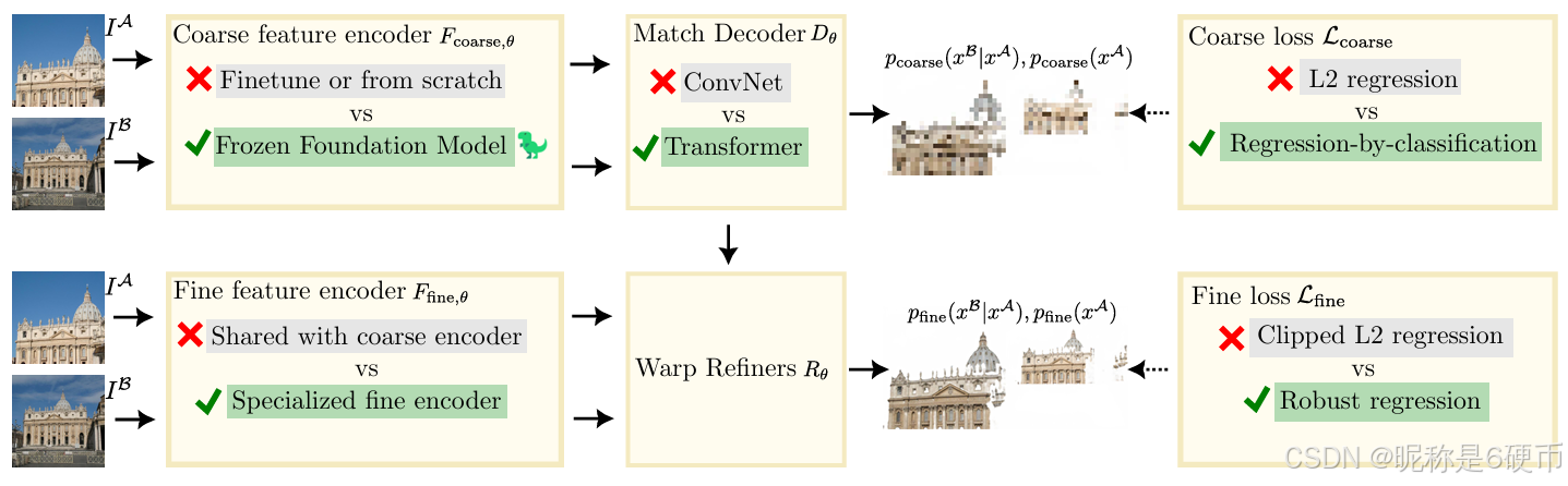
【翻译】图2. 我们的鲁棒方法RoMa的说明。我们的贡献用绿色高亮和勾号显示，而以前的方法用灰色高亮和叉号表示。我们的第一个贡献是使用冻结的基础模型来提取粗糙特征，相比于微调或从头训练。DINOv2缺乏精细特征，而这些特征是准确对应关系所需要的。为了解决这个问题，我们将DINOv2粗糙特征与来自ConvNet的专门精细特征相结合，见第3.2节。第二，我们提出了一个改进的粗糙匹配解码器$D_{\theta }$，它通常是一个ConvNet，使用坐标无关的Transformer解码器，该解码器预测锚点概率而不是直接回归坐标，见第3.3节。第三，我们重新审视了用于密集特征匹配的损失函数。我们从理论模型论证全局匹配阶段需要建模多模态分布，因此使用回归分类损失而不是L2损失。相比之下，对于细化阶段，我们使用鲁棒回归损失，因为匹配分布在局部是单模态的。这些损失在第3.4节中进一步讨论。我们贡献的影响在表2的广泛消融研究中得到验证。

【解析】架构图展示了RoMa方法的三个核心创新点。第一个创新在于特征提取策略的设计：冻结DINOv2作为粗糙特征提取器，同时训练专门的ConvNet来提取精细特征。这种混合策略既利用了大规模预训练模型的泛化能力，又确保了精确的空间定位能力。特征金字塔的构建将不同尺度的信息有机结合，形成了从粗糙到精细的完整特征表示。

第二个创新在于匹配解码器的设计。传统的卷积解码器直接回归坐标值，但这种方法在面对歧义性匹配时容易产生不稳定的结果。Transformer解码器通过预测锚点概率分布来处理这种不确定性，这种概率化的表示能够更好地处理一对多或多对一的匹配情况。坐标无关性说明解码器不依赖于特定的空间位置编码，增强了模型的泛化能力。

第三个创新涉及损失函数设计。在全局匹配阶段，由于特征的粗糙性和场景的复杂性，一个特征点可能对应多个候选匹配点，形成多模态分布。传统的L2损失假设单峰分布，无法有效处理这种多模态性。回归分类损失通过将连续的回归问题转化为离散的分类问题，能够更好地建模多模态分布。而在细化阶段，由于已经有了粗糙匹配的约束，匹配分布变为局部单模态，此时鲁棒回归损失能够有效处理异常值并提供精确的定位。

We overcome this issue by leveraging a frozen DINOv2 encoder for coarse features, while using a proposed specialized ConvNet encoder for the fine features. This has the benefit of incorporating the excellent general features from DINOv2, while simultaneuously having highly precise fine features. We find that features specialized for only coarse matching or refinement significantly outperform features trained for both tasks jointly. These contributions are presented in more detail in Section 3.2. We additionally propose a Transformer match decoder that while also increasing performance for the baseline, particularly improves performance when used to predict anchor probabilities instead of regressing coordinates in conjunction with the DINOv2 coarse encoder. This contribution is elaborated further in Section 3.3.

【翻译】我们通过利用冻结的DINOv2编码器提取粗糙特征，同时使用我们提出的专门的ConvNet编码器提取精细特征来克服这个问题。这样做的好处是结合了DINOv2优秀的通用特征，同时拥有高度精确的精细特征。我们发现专门用于粗糙匹配或细化的特征显著优于为两个任务联合训练的特征。这些贡献在第3.2节中有更详细的介绍。我们还提出了一个Transformer匹配解码器，它不仅提高了基线的性能，特别是在与DINOv2粗糙编码器结合使用时，用于预测锚点概率而不是回归坐标时，性能改善尤为显著。这一贡献在第3.3节中进一步详述。

Lastly, we investigate how to best train dense feature matchers. Recent SotA dense methods such as DKM [17] use a non-robust regression loss for the coarse matching as well as for the refinement. We argue that this is not optimal as the matching distribution at the coarse stage is often multimodal, while the conditional refinement is more likely to be unimodal. Hence requiring different approaches to training. We motivate this from a theoretical framework in Section 3.4. Our framework motivates a division of the coarse and fine losses into seperate paradigms, regressionby-classification for the global matches using coarse features, and robust regression for the refinement using fine features.

【翻译】最后，我们研究如何最好地训练密集特征匹配器。最近的最先进密集方法如DKM [17]在粗糙匹配和细化阶段都使用非鲁棒回归损失。我们认为这不是最优的，因为粗糙阶段的匹配分布通常是多模态的，而条件细化更可能是单模态的。因此需要不同的训练方法。我们在第3.4节从理论框架中论证了这一点。我们的框架促使将粗糙和精细损失划分为不同的范式，对使用粗糙特征的全局匹配使用回归分类，对使用精细特征的细化使用鲁棒回归。

【解析】密集特征匹配训练策略需要考虑到：传统方法在整个匹配流程中使用统一的损失函数，但作者认为这种做法忽略了不同阶段匹配分布的本质差异。在粗糙匹配阶段，由于特征的低分辨率和场景的复杂性，一个特征点可能合理地对应多个候选位置，这形成了多模态分布。例如，在一个重复纹理的场景中，一个粗糙特征可能匹配到多个相似的位置。非鲁棒回归损失（如L2损失）假设单峰分布，在多模态情况下会产生次优的梯度信号。相反，回归分类损失通过离散化候选位置并预测概率分布，能够自然地建模多模态性。在细化阶段，由于已有粗糙匹配的约束和精细特征的高分辨率，匹配分布变为局部单模态，此时鲁棒回归损失能够有效处理异常值并提供精确的定位。

非鲁棒回归损失（如平方损失L2）的单峰假设意味着它假定目标变量围绕真实值呈现单一的高斯分布，即存在一个明确的"正确答案"。这种损失函数计算预测值与真实值之间的欧氏距离，当存在多个合理匹配位置时，会在这些位置之间产生平均化效应，导致模型学习到一个在所有候选位置之间的"妥协"位置，而这个位置可能并不对应任何真实的匹配点。回归分类损失则将连续的坐标回归问题转化为离散的分类问题：首先将二维坐标空间划分为规则网格，每个网格点作为一个类别，然后训练模型预测每个网格点是正确匹配位置的概率。这种方法能够自然地表达多模态分布——多个网格点可以同时具有较高的概率，对应多个合理的匹配候选。在推理时，可以选择概率最高的网格点作为初始匹配，然后在其邻域内进行精细化回归。

Our full approach, which we call RoMa, is robust to extremely challenging real-world cases, as we demonstrate in Figure 1. We illustrate our approach schematically in Figure 2. In summary, our contributions are as follows:

【翻译】我们称之为RoMa的完整方法对极具挑战性的现实世界情况具有鲁棒性，如我们在图1中所展示的。我们在图2中示意性地说明了我们的方法。总结来说，我们的贡献如下：

(a) We integrate frozen features from the foundation model DINOv2 [37] for dense feature matching. We combine the coarse features from DINOv2 with specialized fine features from a ConvNet to produce a precisely localizable yet robust feature pyramid. See Section 3.2.

【翻译】(a) 我们将来自基础模型DINOv2 [37]的冻结特征集成到密集特征匹配中。我们将来自DINOv2的粗糙特征与来自ConvNet的专门精细特征相结合，以产生既精确可定位又鲁棒的特征金字塔。见第3.2节。

【解析】特征金字塔通过组合不同尺度的特征来实现多层次的信息表示。在这里，作者将预训练的DINOv2特征与专门训练的ConvNet特征结合构建特征金字塔。这种设计的核心思想是取长补短：DINOv2特征具有强大的语义理解和泛化能力，能够在各种场景变化下保持稳定的表示，但分辨率相对较低；而专门的ConvNet特征虽然可能缺乏DINOv2那样的泛化能力，但能够提供精确的空间定位信息。作者强调了这种组合既保证了匹配的精度又确保了在复杂环境下的稳定性。

(b) We propose a Transformer-based match decoder, which predicts anchor probabilities instead of coordinates. See Section 3.3.

【翻译】(b) 我们提出了一个基于Transformer的匹配解码器，它预测锚点概率而不是坐标。见第3.3节。

【解析】这个创新点是从确定性预测向概率性预测的转变。传统的匹配解码器直接回归坐标值，这种方法假设每个特征点都有唯一确定的匹配位置。然而，在实际场景中，由于图像噪声、重复纹理、遮挡等因素，匹配往往存在不确定性。锚点概率预测通过将连续的坐标空间离散化为锚点网格，然后预测每个锚点的匹配概率，这种方法能够自然地表达匹配的不确定性和多模态特性（如之前的分析）。Transformer架构特别适合这种概率预测任务，因为其自注意力机制能够捕捉全局的特征关系，帮助模型在复杂场景中做出更可靠的概率判断。

© We improve the loss formulation. In particular, we use a regression-by-classification loss for coarse global matches, while we use robust regression loss for the refinement stage, both of which we motivate from a theoretical analysis. See Section 3.4.

【翻译】© 我们改进了损失函数的表述。特别地，我们对粗糙全局匹配使用回归分类损失，而对细化阶段使用鲁棒回归损失，这两者我们都从理论分析中得出动机。见第3.4节。

【解析】回归分类损失通过概率分布的形式能够保持多峰特性，为后续的细化提供更好的初始化。鲁棒回归损失在细化阶段的使用则是考虑到此时匹配分布已经相对集中，主要需要处理异常值和噪声问题，鲁棒损失函数能够在保证收敛性的同时抑制异常值的影响。

(d) We conduct an extensive ablation study over our contributions, and SotA experiments on a set of diverse and competitive benchmarks, and find that RoMa sets a new state-of-the-art. In particular, achieving a gain of $36\%$ on the difficult $\mathbf{WxBS}$ benchmark. See Section 4.

【翻译】(d) 我们对我们的贡献进行了广泛的消融研究，并在一系列多样化且具有竞争性的基准上进行了最先进的实验，发现RoMa创造了新的最先进水平。特别是，在困难的$\mathbf{WxBS}$基准上取得了$36\%$的提升。见第4节。

2. Related Work

2.1. Sparse $\to$ Detector Free $\to$ Dense Matching

Feature matching has traditionally been approached by keypoint detection and description followed by matching the descriptions [4, 14, 33, 39, 41, 53]. Recently, the detectorfree approach [7, 12, 44, 46] replaces the keypoint detection with dense matching on a coarse scale, followed by mutual nearest neighbors extraction, which is followed by refinement. The dense approach [17, 34, 36, 50, 51, 63] instead estimates a dense warp, aiming to estimate every matchable pixel pair.

【翻译】特征匹配传统上采用关键点检测和描述的方法，然后匹配这些描述 [4, 14, 33, 39, 41, 53]。最近，无检测器方法 [7, 12, 44, 46] 用粗尺度的密集匹配替代关键点检测，随后进行互最近邻提取，然后进行细化。密集方法 [17, 34, 36, 50, 51, 63] 则估计密集扭曲，旨在估计每个可匹配的像素对。

2.2. 自监督视觉模型

Inspired by language Transformers [15] foundation models [8] pre-trained on large quantities of data have recently demonstrated significant potential in learning all-purpose features for various visual models via self-supervised learning. Caron et al. [11] observe that self-supervised ViT features capture more distinct information than supervised models do, which is demonstrated through label-free selfdistillation. iBOT [62] explores MIM within a selfdistillation framework to develop a semantically rich visual tokenizer, yielding robust features effective in various dense downstream tasks. DINOv2 [37] reveals that selfsupervised methods can produce all-purpose visual features that work across various image distributions and tasks after being trained on sufficient datasets without finetuning.

【翻译】受语言Transformers [15]基础模型 [8]的启发，在大量数据上预训练的模型最近通过自监督学习在为各种视觉模型学习通用特征方面展现出巨大潜力。Caron等人 [11]观察到自监督ViT特征比监督模型捕获更独特的信息，这通过无标签自蒸馏得到证明。iBOT [62]在自蒸馏框架内探索MIM以开发语义丰富的视觉标记器，产生在各种密集下游任务中有效的鲁棒特征。DINOv2 [37]揭示了自监督方法能够产生通用视觉特征，这些特征在经过足够数据集训练后，无需微调就能在各种图像分布和任务中工作。

【解析】自监督学习的核心思想是让模型从无标签数据中学习有用的表示，而不依赖人工标注。这一领域的演进：首先，Caron等人发现自监督的ViT特征相比监督学习的特征能够捕获更多独特信息，这种优势通过自蒸馏技术得到验证——自蒸馏是一种让模型向自己学习的技术，通过预测一个视图的特征来匹配另一个视图的特征。iBOT进一步发展了这一思路，将掩码图像建模（MIM）与自蒸馏结合，创建了语义丰富的视觉标记器，这种方法通过重建被掩盖的图像片段来学习特征表示。DINOv2则代表了自监督学习的一个重要里程碑，它证明了在足够大的数据集上训练的自监督模型可以产生真正的通用视觉特征，这些特征无需针对特定任务进行微调就能在不同的图像分布和各种视觉任务中表现良好。这种通用性对于特征匹配任务特别有价值，因为它说明预训练的DINOv2特征具有强大的跨域泛化能力，能够处理各种场景和视觉条件下的图像匹配问题。

2.3. 鲁棒损失函数表述

Robust Regression Losses: Robust loss functions provide a continuous transition between an inlier distribution (typically highly concentrated), and an outlier distribution (wide and flat). Robust losses have, e.g., been used as regularizers for optical flow [5, 6], robust smoothing [18], and as loss functions [3, 32].

【翻译】鲁棒回归损失：鲁棒损失函数在内点分布（通常高度集中）和异常点分布（宽泛且平坦）之间提供连续过渡。鲁棒损失已被用作光流的正则化器 [5, 6]、鲁棒平滑 [18]，以及损失函数 [3, 32]。

【解析】鲁棒损失函数的核心设计理念是能够区分并适应不同类型的数据点分布特性。内点分布通常表现为围绕真实值的高度集中分布，这些点代表了可靠的观测数据，应该给予较大的权重；而异常点分布则表现为宽泛且平坦的分布，这些点可能由于噪声、遮挡或错误测量产生，应该被抑制其影响。传统的L2损失对所有点都给予相同的二次惩罚，这使得异常值会对模型产生过大的影响，因为其误差的平方会被放大。鲁棒损失函数通过设计非线性的惩罚机制，在误差较小时提供类似于L2的行为以保证精度，而在误差较大时则提供更温和的惩罚以减少异常值的影响。这种连续过渡的特性使得损失函数在优化过程中能够平滑地处理不同质量的数据点，既保证了对高质量数据的敏感性，又具备了对低质量数据的鲁棒性。在光流估计、图像平滑和特征匹配等计算机视觉任务中，这种特性尤其重要，因为这些任务经常面临噪声、遮挡和运动边界等挑战。

Regression by Classification: Regression by classification [48, 57, 58] involves casting regression problems as classification by, e.g., binning. This is particularly useful for regression problems with sharp borders in motion, such as stereo disparity [19, 22]. Germain et al. [20] use a regression-by-classification loss for absolute pose regression.

【翻译】回归分类：回归分类 [48, 57, 58] 涉及通过例如分箱的方式将回归问题转换为分类问题。这对于具有运动尖锐边界的回归问题特别有用，例如立体视差 [19, 22]。Germain等人 [20] 使用回归分类损失进行绝对姿态回归。

【解析】回归分类的核心思想是将连续的回归目标空间离散化为有限个类别，然后使用分类框架来解决原本的回归问题。这种方法的优势在于能够处理多模态分布和不连续性问题。在传统回归中，模型假设输出是连续的并且存在唯一的最优解，但在许多计算机视觉任务中，这种假设并不成立。例如，在立体视差估计中，由于遮挡、重复纹理或反射表面的存在，一个像素可能对应多个合理的视差值，形成多峰分布。分箱策略将连续的视差范围划分为离散的区间，每个区间作为一个类别，模型预测每个类别的概率而不是直接预测数值。这种方法的另一个重要优势是能够自然地表达预测的不确定性：高熵的概率分布表示高不确定性，而集中的概率分布表示高置信度。

Classification then Regression: Li et al. [27], and Budvytis et al. [9] proposed hierarchical classificationregression frameworks for visual localization. Sun et al. [44] optimize the model log-likelihood of mutual nearest neighbors, followed by L2 regression-based refinement for feature matching.

【翻译】分类后回归：Li等人 [27] 和Budvytis等人 [9] 为视觉定位提出了分层分类回归框架。Sun等人 [44] 优化互最近邻的模型对数似然，然后进行基于L2回归的细化以进行特征匹配。

【解析】分类后回归策略采用了层次化的粗到细的处理方式，充分利用了分类和回归各自的优势。在第一阶段，分类器用于处理大范围的搜索空间和多模态分布问题，它能够快速识别出最有可能的候选区域或类别，有效地缩小了搜索范围。这个阶段特别适合处理全局性的匹配问题，因为分类框架能够同时考虑多个可能的匹配候选，而不会像直接回归那样产生平均化效应。在第二阶段，回归器在分类器确定的局部区域内进行精细化处理，此时由于搜索空间已经大幅缩小且分布相对单一，传统的回归方法能够发挥其精确定位的优势。Sun等人的方法展示了这种策略在特征匹配中的具体应用：首先通过优化互最近邻的对数似然来建立粗糙的匹配关系，这个过程本质上是一个软分类过程，能够处理匹配的多义性和不确定性；然后使用L2回归损失在确定的匹配邻域内进行精确的坐标细化。这种两阶段设计不仅提高了匹配的准确性，还增强了算法对复杂场景的适应能力，因为它能够在保持全局搜索能力的同时实现局部的精确定位（关于这个方法的使用可以参考Patch2Pix，Patch2Pix论文精读（逐行解析）链接待补充）。

3. Method

In this section, we detail our method. We begin with preliminaries and notation for dense feature matching in Section 3.1. We then discuss our incorporation of DINOv2 [37] as a coarse encoder, and specialized fine features in Section 3.2. We present our proposed Transformer match decoder in Section 3.3. Finally, our proposed loss formulation in Section 3.4. A summary and visualization of our full approach is provided in Figure 2. Further details on the exact architecture are given in the supplementary.

【翻译】在本节中，我们详细介绍我们的方法。我们首先在第3.1节介绍密集特征匹配的基础知识和符号表示。然后在第3.2节讨论我们如何将DINOv2 [37]作为粗糙编码器，以及专门的精细特征。我们在第3.3节展示我们提出的Transformer匹配解码器。最后，在第3.4节介绍我们提出的损失函数表述。图2提供了我们完整方法的总结和可视化。关于具体架构的进一步细节在补充材料中给出。

3.1. 密集特征匹配的基础知识

Dense feature matching is, given two images $I^A,I^B$ , to estimate a dense warp $W^{\mathbf{A}\to B}$ (mapping coordinates $x^A$ from $I^A$ to $x^B$ in $I^{\mathbf{B}}$ ), and a matchability score $p(x^A)$ for each pixel. From a probabilistic perspective, $p(W^{A\to B})=p(x^B|x^A)$ is the conditional matching distribution. Multiplying $p(x^B|x^A)p(x^A)$ yields the joint distribution. We denote the model distribution as $p_{\theta }(x^A,x^B)=$ $p_{\theta }(x^B|x^A)p_{\theta }(x^A)$ . When working with warps, i.e., where $p_{\theta }(x^B|x^A)$ has been converted to a deterministic mapping, we denote the model warp as ${\hat{W}}^{A\to B}$ . Viewing the predictive distribution as a warp is natural in high resolution, as it can then be seen as a deterministic mapping. However, due to multimodality, it is more natural to view it in the probabilistic sense at coarse scales.

【翻译】密集特征匹配是指，给定两张图像$I^A,I^B$，估计一个密集扭曲$W^{\mathbf{A}\to B}$（将坐标$x^A$从$I^A$映射到$I^{\mathbf{B}}$中的$x^B$），以及每个像素的可匹配性分数$p(x^A)$。从概率角度来看，$p(W^{A\to B})=p(x^B|x^A)$是条件匹配分布。将$p(x^B|x^A)p(x^A)$相乘得到联合分布。我们将模型分布表示为$p_{\theta }(x^A,x^B)=$ $p_{\theta }(x^B|x^A)p_{\theta }(x^A)$。当处理扭曲时，即$p_{\theta }(x^B|x^A)$被转换为确定性映射时，我们将模型扭曲表示为${\hat{W}}^{A\to B}$。在高分辨率下将预测分布视为扭曲是自然的，因为这时可以将其视为确定性映射。然而，由于多模态性，在粗糙尺度下将其视为概率意义更自然。

【解析】密集特征匹配可以用数学上的扭曲函数$W^{A\to B}$来描述，它将图像A中的坐标映射到图像B中的坐标。可匹配性分数$p(x^A)$评估每个像素是否有合理的匹配对象，这对于处理遮挡、出界或无纹理区域非常重要。从概率论的角度，条件分布$p(x^B|x^A)$描述了给定图像A中一个像素位置时，它在图像B中对应位置的概率分布。联合分布$p(x^A,x^B)$则通过链式法则将边缘分布和条件分布结合起来，完整描述了两个像素位置的联合概率。模型在不同分辨率下采用不同的表示方式：在高分辨率下，每个像素通常有唯一的最佳匹配，因此可以用确定性的扭曲函数来表示；而在低分辨率下，由于信息的模糊性和多种可能的匹配情况，概率分布的表示更能反映匹配的不确定性和多模态特性。

The end goal is to obtain a good estimate over correspondences of coordinates $x^A$ in image $I^A$ and coordinates $x^B$ in image $I^{\mathbf{B}}$ . For dense feature matchers, estimation of these correspondences is typically done by a one-shot coarse global matching stage (using coarse features) followed by subsequent refinement of the estimated warp and confidence (using fine features).

【翻译】最终目标是获得图像$I^A$中坐标$x^A$与图像$I^{\mathbf{B}}$中坐标$x^B$之间对应关系的良好估计。对于密集特征匹配器，这些对应关系的估计通常通过一次性粗糙全局匹配阶段（使用粗糙特征）完成，随后对估计的扭曲和置信度进行细化（使用精细特征）。

【解析】密集特征匹配采用了分层次的粗到细策略来解决复杂的对应关系估计问题。第一阶段的粗糙全局匹配负责建立大致的对应关系，这个阶段使用低分辨率的粗糙特征来减少计算复杂度，同时能够捕获图像间的整体变换关系。粗糙特征虽然缺乏精确的空间定位能力，但具有较大的感受野和丰富的语义信息，适合处理大尺度的变形和视点变化。第二阶段的细化过程则在粗糙匹配的基础上，使用高分辨率的精细特征来提高匹配的精度。精细特征具有更好的空间定位能力，能够捕获细微的纹理和边缘信息，从而实现像素级的精确匹配。这种两阶段设计既保证了算法的效率（粗糙阶段减少搜索空间），又确保了匹配的精度（细化阶段提供精确定位），同时置信度的估计帮助识别和过滤不可靠的匹配结果。

We use the recent SotA dense feature matching model DKM [17] as our baseline. For consistency, we adapt the terminology used there. We denote the coarse features used to estimate the initial warp, and the fine features used to refine the warp by

{φcoarseA,φfineA}=Fθ(IA),{φcoarseB,φfineB}=Fθ(IB),\{\varphi_{\mathrm{coarse}}^{A},\varphi_{\mathrm{fine}}^{A}\}=F_{\theta}(I^{A}),\{\varphi_{\mathrm{coarse}}^{B},\varphi_{\mathrm{fine}}^{B}\}=F_{\theta}(I^{B}), {φcoarseA​,φfineA​}=Fθ​(IA),{φcoarseB​,φfineB​}=Fθ​(IB),

where $F_{\theta }$ is a neural network feature encoder. We will leverage DINOv2 for extraction of ${\phi }_{\mathrm{coarse}}^A,{\phi }_{\mathrm{coarse}}^B$, however, DINOv2 features are not precisely localizable, which we tackle by combining the coarse features with precise local features from a specialized ConvNet backbone. See Section 3.2 for details.

【翻译】我们使用最近的最先进密集特征匹配模型DKM [17]作为我们的基线。为了一致性，我们采用其中使用的术语。我们用以下方式表示用于估计初始扭曲的粗糙特征和用于细化扭曲的精细特征：

其中$F_{\theta }$是神经网络特征编码器。我们将利用DINOv2来提取${\phi }_{\mathrm{coarse}}^A,{\phi }_{\mathrm{coarse}}^B$，然而，DINOv2特征不能精确定位，我们通过将粗糙特征与来自专门的ConvNet骨干网络的精确局部特征相结合来解决这个问题。详见第3.2节。

【解析】这里建立了特征提取的框架。特征编码器$F_{\theta }$是一个参数化的神经网络，它将输入图像映射到多层次的特征表示空间。DINOv2作为自监督训练的Vision Transformer，在大规模数据上学习到了强大的视觉表示能力，其特征具有很好的语义表达能力和跨域泛化性，非常适合作为粗糙特征来处理复杂的匹配场景。然而，DINOv2的patch-based架构导致其特征缺乏像素级的精确定位能力，这正是传统卷积网络的优势所在。因此，作者设计了混合架构，利用DINOv2的语义理解能力和卷积网络的精确定位能力，实现了功能互补。

The coarse features are matched with global matcher $G_{\theta }$ consisting of a match encoder $E_{\theta }$ and match decoder $D_{\theta }$ ,

$$\begin{array}{r}\{\begin{array}{l}({\hat{\mathbf{W}}}_{\mathrm{coarse}}^{A\to B},p_{\theta ,\mathrm{coarse}}^A)=G_{\theta }({\phi }_{\mathrm{coarse}}^A,{\phi }_{\mathrm{coarse}}^B),\\ G_{\theta }({\phi }_{\mathrm{coarse}}^A,{\phi }_{\mathrm{coarse}}^B)=D_{\theta }(E_{\theta }({\phi }_{\mathrm{coarse}}^A,{\phi }_{\mathrm{coarse}}^B)).\end{array}\end{array}$$

【翻译】粗糙特征通过全局匹配器$G_{\theta }$进行匹配，该匹配器由匹配编码器$E_{\theta }$和匹配解码器$D_{\theta }$组成，

【解析】这里定义了粗糙特征匹配的架构。全局匹配器$G_{\theta }$是一个复合函数，它将两张图像的粗糙特征${\phi }_{\mathrm{coarse}}^A$和${\phi }_{\mathrm{coarse}}^B$作为输入，输出粗糙层次的扭曲估计${\hat{\mathbf{W}}}_{\mathrm{coarse}}^{A\to B}$和可匹配性概率$p_{\theta ,\mathrm{coarse}}^A$。这个过程被分解为两个连续的步骤：首先匹配编码器$E_{\theta }$处理输入的特征对，生成中间表示；然后匹配解码器$D_{\theta }$将这个中间表示转换为最终的匹配结果。

We use a Gaussian Process [38] as the match encoder $E_{\theta }$ as in previous work [17]. However, while our baseline uses a ConvNet to decode the matches, we propose a Transformer match decoder $D_{\theta }$ that predicts anchor probabilities instead of directly regressing the warp. This match decoder is particularly beneficial in our final approach (see Table 2). We describe our proposed match decoder in Section 3.3. The refinement of the coarse warp ${\hat{\mathbf{W}}}_{\mathrm{coarse}}^{\mathcal{A}\to B}$ Vcoarse is done by the refiners $R_{\theta }$ ,

【翻译】我们像之前的工作[17]一样使用高斯过程[38]作为匹配编码器$E_{\theta }$。然而，虽然我们的基线使用ConvNet来解码匹配，但我们提出了一个Transformer匹配解码器$D_{\theta }$，它预测锚点概率而不是直接回归扭曲。这个匹配解码器在我们的最终方法中特别有益（见表2）。我们在第3.3节中描述我们提出的匹配解码器。粗糙扭曲${\hat{\mathbf{W}}}_{\mathrm{coarse}}^{\mathcal{A}\to B}$的细化由细化器$R_{\theta }$完成，

【解析】这里说明了作者在匹配解码器设计上的创新。高斯过程作为匹配编码器能够有效地建模特征之间的相关性和不确定性，这是其在之前工作中被证明有效的原因。关键的创新在于匹配解码器的设计：传统的卷积网络解码器直接回归扭曲参数，这种方法假设存在唯一的最优解，但在实际的匹配场景中，由于遮挡、重复纹理等因素，一个位置可能对应多个合理的匹配候选。作者提出的Transformer解码器采用了回归分类的策略，通过预测离散锚点的概率分布而不是直接回归连续的扭曲值。这种设计能够自然地处理匹配的多模态性和不确定性，Transformer的自注意力机制也使得模型能够更好地捕获全局的上下文信息，从而提升匹配的准确性。细化器$R_{\theta }$则负责在粗糙匹配的基础上进行精确调整，实现从粗到细的层次化匹配策略。

$$({\hat{\mathbf{W}}}^{\mathcal{A}\to \mathcal{B}},p_{\theta }^{\mathcal{A}})=R_{\theta }({\phi }_{\mathrm{fine}}^{\mathcal{A}},{\phi }_{\mathrm{fine}}^{\mathcal{B}},{\hat{\mathbf{W}}}_{\mathrm{coarse}}^{\mathcal{A}\to \mathcal{B}},p_{\theta ,\mathrm{coarse}}^{\mathcal{A}}).$$

【解析】这个公式定义了细化器的输入输出关系。细化器$R_{\theta }$接受四个输入：两张图像的精细特征${\phi }_{\mathrm{fine}}^{\mathcal{A}}$和${\phi }_{\mathrm{fine}}^{\mathcal{B}}$、粗糙层次的扭曲估计${\hat{\mathbf{W}}}_{\mathrm{coarse}}^{\mathcal{A}\to \mathcal{B}}$以及粗糙层次的可匹配性概率$p_{\theta ,\mathrm{coarse}}^{\mathcal{A}}$。输出是最终的精细扭曲${\hat{\mathbf{W}}}^{\mathcal{A}\to \mathcal{B}}$和更新后的可匹配性概率$p_{\theta }^{\mathcal{A}}$。这种设计使得细化器能够充分利用多层次的信息：精细特征提供高分辨率的局部细节，粗糙扭曲提供全局的几何约束，而可匹配性概率则指导细化过程关注那些更可能有正确匹配的区域。

As in previous work, the refiner is composed of a sequence of ConvNets (using strides {1,2,4,8}.\{1,2,4,8\}.{1,2,4,8}. ) and can be decomposed recursively as

$$\begin{array}{r}({\hat{W}}_i^{\mathcal{A}\to \mathcal{B}},p_{i,\mathbf{\theta }}^{\mathcal{A}})=R_{\mathbf{\theta },i}({\phi }_i^{\mathcal{A}},{\phi }_i^{\mathcal{B}},{\hat{W}}_{i+1}^{\mathcal{A}\to \mathcal{B}},p_{\mathbf{\theta },i+1}^{\mathcal{A}}),\end{array}$$

【翻译】如在之前的工作中，细化器由一系列ConvNets组成（使用步长{1,2,4,8}.\{1,2,4,8\}.{1,2,4,8}.），并且可以递归分解为

【解析】这里定义了细化器的内部结构和递归计算过程。细化器采用多尺度的金字塔结构，通过不同步长（{1,2,4,8}\{1,2,4,8\}{1,2,4,8}）的卷积网络来处理不同分辨率的特征。递归公式显示了细化过程是一个从粗到细的迭代过程：每个细化阶段$R_{\mathbf{\theta },i}$都依赖于当前尺度的特征${\phi }_i^{\mathcal{A}}$、${\phi }_i^{\mathcal{B}}$以及来自上一个（更粗糙）尺度的扭曲估计${\hat{W}}_{i+1}^{\mathcal{A}\to \mathcal{B}}$和可匹配性概率$p_{\mathbf{\theta },i+1}^{\mathcal{A}}$。这种递归设计使得每个细化阶段都能在前一阶段的基础上进行增量改进，逐步提高匹配的精度。步长是图像金字塔的标准设计，即其中每一层的分辨率都是前一层的两倍。

where the stride is $2^i$ . The refiners predict a residual offset for the estimated warp, and a logit offset for the certainty. As in the baseline they are conditioned on the outputs of the previous refiner by using the previously estimated warp to a) stack feature maps from the images, and b) construct a local correlation volume around the previous target.

【翻译】其中步长是$2^i$。细化器预测估计扭曲的残差偏移量，以及确定性的logit偏移量。如在基线中一样，它们通过使用先前估计的扭曲来a）堆叠来自图像的特征图，和b）在先前目标周围构建局部相关体积，从而依赖于先前细化器的输出。

【解析】步长$2^i$是多尺度处理的思路，其中$i$越小，分辨率越高。细化器采用残差学习的思想，不是直接预测最终的扭曲值，而是预测相对于前一阶段估计的残差偏移量，这种设计使得学习过程更加稳定且容易收敛。对于确定性的预测，模型输出logit偏移量而不是直接的概率值，这样可以更好地控制数值稳定性。条件化机制是细化器能够有效工作的关键：首先，通过堆叠特征图，模型能够同时访问两张图像在当前位置的特征信息；其次，局部相关体积的构建限制了搜索范围，减少了计算复杂度同时避免了错误匹配，这个体积是在前一阶段预测的目标位置周围的局部区域内计算特征相关性。

The process is repeated until reaching full resolution. We use the same architecture as in the baseline. Following DKM, we detach the gradients between the refiners and upsample the warp bilinearly to match the resolution of the finer stride.

【翻译】这个过程重复进行直到达到完整分辨率。我们使用与基线相同的架构。遵循DKM，我们在细化器之间分离梯度，并双线性上采样扭曲以匹配更精细步长的分辨率。

【解析】整个细化是一个多尺度的迭代过程，从最粗糙的分辨率开始，逐步细化到原始图像的完整分辨率。梯度分离是训练策略的关键设计：在不同细化器之间切断梯度传播可以防止梯度爆炸或消失问题，同时让每个细化器专注于自己尺度的任务，避免不同尺度之间的相互干扰。双线性上采样是分辨率匹配的标准方法，当从一个粗糙的扭曲估计转到更精细的尺度时，需要将扭曲场的空间分辨率相应提升，双线性插值提供了平滑且计算高效的上采样方式，确保扭曲场在不同尺度间的连续性。

【扭曲场的几何含义】关于本文中反复提到的"扭曲场"（warp field），需要明确其与传统单应性矩阵（H矩阵）的区别。传统的图像匹配方法通常假设两幅图像之间存在全局的平面单应性变换，可以用3×3的单应性矩阵H来描述，这种表示方式简洁但只适用于平面场景或视角变化较小的情况。而本文中的扭曲场是一个更加通用和灵活的几何变换表示：它是一个密集的空间变换场，为图像中每个像素位置$(x,y)$都定义了其在目标图像中的对应位置$(x^{\prime },y^{\prime })$。这种表示能够处理任意复杂的非刚性变形，包括透视变换、非平面3D结构引起的视差、局部变形等。扭曲场实际上是H矩阵的泛化：当场景为完美平面且视角变化符合单应性假设时，扭曲场会退化为全局一致的单应性变换；但在复杂的真实场景中，扭曲场能够编码更丰富的几何关系，使得匹配模型具有更强的适应性和鲁棒性。

Probabilistic Notation: When later defining our loss functions, it will be convenient to refer to the outputs of the different modules in a probabilistic notation. We therefore introduce this notation here first for clarity.

【翻译】概率记号：当稍后定义我们的损失函数时，用概率记号来指代不同模块的输出将会很方便。因此我们首先在这里介绍这个记号以保持清晰。

【解析】同一个特征点可能有多个合理的匹配候选，或者由于遮挡、模糊等因素导致匹配的置信度不同。采用概率表示能够自然地建模这种不确定性，让模型输出不再是单一的确定值，而是概率分布。这种概率框架为设计更sophisticated的损失函数提供了数学基础，使得训练过程能够更好地处理匹配的多模态性和不确定性。

We denote the probability distribution modeled by the global matcher as

$$p_{\theta }(x_{\mathrm{coarse}}^{\mathcal{A}},x_{\mathrm{coarse}}^{\mathcal{B}})=G_{\theta }({\phi }_{\mathrm{coarse}}^{\mathcal{A}},{\phi }_{\mathrm{coarse}}^{\mathcal{B}}).$$

【翻译】我们将全局匹配器建模的概率分布表示为

【解析】这个公式建立了全局匹配器输出的概率解释。$p_{\theta }(x_{\mathrm{coarse}}^{\mathcal{A}},x_{\mathrm{coarse}}^{\mathcal{B}})$表示图像$\mathcal{A}$中位置$x_{\mathrm{coarse}}^{\mathcal{A}}$和图像$\mathcal{B}$中位置$x_{\mathrm{coarse}}^{\mathcal{B}}$之间的联合概率分布。联合分布的表示方式比传统的条件概率$p(x^{\mathcal{B}}|x^{\mathcal{A}})$更加通用，它不仅表达匹配的方向性，还能捕捉双向匹配的一致性约束。全局匹配器$G_{\theta }$通过处理两张图像的粗糙特征，直接输出这个联合概率分布，这个分布编码了在粗糙尺度上所有可能的匹配关系及其置信度。

Here we have dropped the explicit dependency on the features and the previous estimate of the marginal for notational brevity. Note that the output of the global matcher will sometimes be considered as a discretized distribution using anchors, or as a decoded warp. We do not use separate notation for these two different cases to keep the notation uncluttered.

【翻译】这里我们为了记号简洁性省略了对特征和先前边际估计的显式依赖。注意全局匹配器的输出有时会被视为使用锚点的离散化分布，或者作为解码的扭曲。我们不对这两种不同情况使用单独的记号以保持记号简洁。

【解析】在完整的表示中，概率分布应该显式地依赖于输入特征${\phi }_{\mathrm{coarse}}^{\mathcal{A}},{\phi }_{\mathrm{coarse}}^{\mathcal{B}}$，但为了避免记号过于复杂，这里采用了简化表示。更重要的是，全局匹配器的输出具有双重性质：在训练阶段，它可能以离散锚点概率分布的形式存在，这种表示便于计算分类损失；在推理阶段，它需要被解码为连续的扭曲场，用于后续的细化过程。

We denote the probability distribution modeled by a refiner at scale $s=c{2}^i$ as

$$p_{\theta }(x_i^{\mathcal{A}},x_i^{\mathcal{B}}|{\hat{W}}_{i+1}^{\mathcal{A}\to \mathcal{B}})=R_{\theta ,i}({\phi }_i^{\mathcal{A}},{\phi }_i^{\mathcal{B}},{\hat{W}}_{i+1}^{\mathcal{A}\to \mathcal{B}},p_{\theta ,i+1}^{\mathcal{A}}),$$

【翻译】我们将细化器在尺度$s=c{2}^i$上建模的概率分布表示为

【解析】这个公式定义了细化器在特定尺度上的概率建模方式。$s=c{2}^i$建立了多尺度处理的数学框架，其中$c$是基础常数，$i$是尺度索引，随着$i$的减小，分辨率逐渐提高。关键在于条件概率的设计：$p_{\theta }(x_i^{\mathcal{A}},x_i^{\mathcal{B}}|{\hat{W}}_{i+1}^{\mathcal{A}\to \mathcal{B}})$表示在给定上一尺度扭曲估计${\hat{W}}_{i+1}^{\mathcal{A}\to \mathcal{B}}$的条件下，当前尺度的匹配概率分布。细化器$R_{\theta ,i}$的输入包括当前尺度的特征、前一尺度的扭曲估计和可匹配性概率，丰富的输入信息使得细化过程能够充分利用多层次的先验知识。

The basecase ${\hat{W}}_{\mathrm{coarse}}^{\mathcal{A}\to B}$ is computed by decoding $p_{\theta }(x_{\mathrm{coarse}}^B|x_{\mathrm{coarse}}^A)$. As for the global matcher we drop the explicit dependency on the features.

【翻译】基础情况${\hat{W}}_{\mathrm{coarse}}^{\mathcal{A}\to B}$通过解码$p_{\theta }(x_{\mathrm{coarse}}^B|x_{\mathrm{coarse}}^A)$来计算。与全局匹配器一样，我们省略对特征的显式依赖。

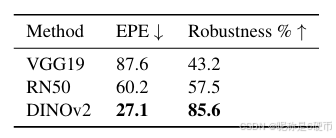
Table 1. Evaluation of frozen features on MegaDepth. We compare the VGG19 and ResNet50 backbones commonly used in feature matching with the generalist features of DINOv2.

【翻译】表1. 在MegaDepth上对冻结特征的评估。我们比较了在特征匹配中常用的VGG19和ResNet50骨干网络与DINOv2的通用特征。

3.2. 鲁棒和可定位的特征

We first investigate the robustness of DINOv2 to viewpoint and illumination changes compared to VGG19 and ResNet50 on the MegaDepth [28] dataset. To decouple the backbone from the matching model we train a single linear layer on top of the frozen model followed by a kernel nearest neighbour matcher for each method. We measure the performance both in average end-point-error (EPE) on a standardized resolution of $448\times 448$ , and by what we call the Robustness $\%$ which we define as the percentage of matches with an error lower than 32 pixels. We refer to this as robustness, as, while these matches are not necessarily accurate, it is typically sufficient for the refinement stage to produce a correct adjustment.

【翻译】我们首先在MegaDepth数据集上研究DINOv2相比VGG19和ResNet50对视角和光照变化的鲁棒性。为了将骨干网络与匹配模型解耦，我们在每种方法的冻结模型之上训练一个单线性层，然后接一个核最近邻匹配器。我们在$448\times 448$的标准化分辨率上同时测量平均端点误差（EPE）和我们称为鲁棒性%的性能，后者定义为误差低于32像素的匹配百分比。我们将其称为鲁棒性，因为虽然这些匹配不一定准确，但通常足以让细化阶段产生正确的调整。

【解析】这个实验设计的目的其实是公平比较不同预训练特征的内在鲁棒性。通过在冻结特征之上只添加简单的线性层，避免复杂匹配架构对比较结果的干扰，让实验重点聚焦在特征本身的质量差异上。端点误差（EPE）是传统的精度指标，衡量预测匹配点与真实匹配点之间的欧几里得距离。而鲁棒性%这个新指标更关注匹配的可用性：在图像匹配的粗到细流水线中，粗糙阶段的匹配不需要像素级精度，只要能提供足够好的初始化，细化阶段就能将其修正到高精度。32像素的阈值是一个经验值，它是典型细化算法的收敛半径：即从多远的初始估计开始，细化过程仍能成功收敛到正确匹配。

We present results in Table 1. We find that DINOv2 features are significantly more robust to changes in viewpoint than both ResNet and VGG19. Interestingly, we find that the VGG19 features are worse than the ResNet features for coarse matching, despite VGG feature being widely used as local features [16, 42, 52]. Further details of this experiment are provided in the supplementary material.

【翻译】我们在表1中展示结果。我们发现DINOv2特征对视角变化的鲁棒性显著优于ResNet和VGG19。有趣的是，我们发现VGG19特征在粗糙匹配中表现比ResNet特征更差，尽管VGG特征被广泛用作局部特征。这个实验的更多细节在补充材料中提供。

【解析】大视角变化下也是DINOv2最强。

In DKM [17], the feature encoder $F_{\theta }$ is assumed to consist of a single network producing a feature pyramid of coarse and fine features used for global matching and refinement respectively. This is problematic when using DINOv2 features as only features of stride 14 exist. We therefore decouple $F_{\theta }$ into {Fcoarse,θ,Ffine,θ}\{F_{\mathrm{coarse},\theta},F_{\mathrm{fine},\theta}\}{Fcoarse,θ​,Ffine,θ​} and set $F_{\mathrm{coarse},\theta }=$ DINOv2. The coarse features are extracted as

【翻译】在DKM中，特征编码器$F_{\theta }$被假设由单个网络组成，产生用于全局匹配和细化的粗糙和精细特征金字塔。当使用DINOv2特征时这变得有问题，因为只存在步长为14的特征。因此我们将$F_{\theta }$解耦为{Fcoarse,θ,Ffine,θ}\{F_{\mathrm{coarse},\theta},F_{\mathrm{fine},\theta}\}{Fcoarse,θ​,Ffine,θ​}并设置$F_{\mathrm{coarse},\theta }=$ DINOv2。粗糙特征提取如下：

【解析】DKM的原始设计假设单一网络能够同时产生适合不同任务的多尺度特征，这种设计在使用传统CNN时是可行的，因为CNN天然具有层次化的特征金字塔结构。然而，DINOv2作为Vision Transformer架构，其设计理念与CNN根本不同：它只输出固定步长（stride 14）的特征图，无法直接提供传统意义上的多尺度特征金字塔。步长14$\approx$输出特征图的空间分辨率是输入图像的1/14，这种相对粗糙的分辨率适合捕捉全局语义信息，但不足以支持精确的像素级匹配细化。解耦设计的思想：让$F_{\mathrm{coarse},\theta }$专注于提供鲁棒的全局语义特征，而$F_{\mathrm{fine},\theta }$专注于提供高分辨率的定位特征。

$$\begin{array}{r}{\phi }_{\mathrm{coarse}}^{\mathbf{A}}=F_{\mathrm{coarse},\mathbf{\theta }}({\mathbf{I}}^{\mathbf{A}}),{\phi }_{\mathrm{coarse}}^{\mathbf{B}}=F_{\mathrm{coarse},\mathbf{\theta }}({\mathbf{I}}^{\mathbf{B}}).\end{array}$$

We keep the DINOv2 encoder frozen throughout training. This has two benefits. The main benefit is that keeping the representations fixed reduces overfitting to the training set, enabling RoMa to be more robust. It is also additionally significantly cheaper computationally and requires less memory. However, DINOv2 cannot provide fine features. Hence a choice of $F_{\mathrm{fine},\theta }$ is needed. While the same encoder for fine features as in DKM could be chosen, i.e., a ResNet50 (RN50) [23], it turns out that this is not optimal.

【翻译】我们在整个训练过程中保持DINOv2编码器冻结。这有两个好处。主要好处是保持表示固定可以减少对训练集的过拟合，使RoMa更加鲁棒。此外，这在计算上也显著更便宜且需要更少的内存。然而，DINOv2无法提供精细特征。因此需要选择$F_{\mathrm{fine},\theta }$。虽然可以选择与DKM中精细特征相同的编码器，即ResNet50 (RN50)，但事实证明这并不是最优的。

We begin by investigating what happens by simply decoupling the coarse and fine feature encoder, i.e., not sharing weights between the coarse and fine encoder (even when using the same network). We find that, as supported by Setup II in Table 2, this significantly increases performance. This is due to the feature extractor being able to specialize in the respective tasks, and hence call this specialization.

【翻译】我们首先研究通过简单地解耦粗糙和精细特征编码器会发生什么，即不在粗糙和精细编码器之间共享权重（即使使用相同的网络）。我们发现，如表2中Setup II所支持的，这显著提高了性能。这是由于特征提取器能够专门化于各自的任务，因此我们称之为专门化。

【解析】作者测试了权重解耦的设计：传统的做法是让单一网络同时处理粗糙匹配和精细匹配任务，通过共享低层特征来提高参数效率。然而，这种共享可能导致特征表示的妥协：粗糙匹配需要的是对大尺度几何变换和语义变化鲁棒的全局特征，而精细匹配需要的是能够精确定位边缘和纹理细节的局部特征。当两个编码器独立优化时，每个编码器可以完全专注于自己的任务目标，学习最适合该任务的特征表示。

This raises a question, VGG19 features, while less suited for coarse matching (see Table 1), could be better suited for fine localized features. We investigate this by setting $F_{\mathrm{fine},\theta }=VGG19$ in Setup III in Table 2. Interestingly, even though VGG19 coarse features are significantly worse than RN50, we find that they significantly outperform the RN50 features when leveraged as fine features. Our finding indicates that there is an inherent tension between fine localizability and coarse robustness. We thus use VGG19 fine features in our full approach.

【翻译】这提出了一个问题，VGG19特征虽然不太适合粗糙匹配（见表1），但可能更适合精细定位特征。我们通过在表2的Setup III中设置$F_{\mathrm{fine},\theta }=VGG19$来研究这一点。有趣的是，尽管VGG19粗糙特征明显比RN50差，但我们发现当用作精细特征时，它们显著优于RN50特征。我们的发现表明精细定位能力和粗糙鲁棒性之间存在内在张力。因此我们在完整方法中使用VGG19精细特征。

3.3. Transformer匹配解码器 $D_{\theta }$

Regression-by-Classification: We propose to use the regression by classification formulation for the match decoder, whereby we discretize the output space. We choose the following formulation,

【翻译】回归分类化：我们提出对匹配解码器使用回归分类化公式，通过离散化输出空间。我们选择以下公式：

【解析】传统的图像匹配方法通常将匹配问题视为回归任务，直接预测连续的坐标值。然而，这种连续回归方法在处理复杂场景时容易产生模糊的预测，特别是在存在重复纹理或遮挡的情况下。回归分类化将连续预测问题转换为离散分类问题：不直接预测精确的坐标值，而是预测属于预定义网格位置的概率分布。

$$p_{\mathrm{coarse},\theta }(x^{\mathcal{B}}|x^{\mathcal{A}})=\sum _{k=1}^K{\pi }_k(x^{\mathcal{A}}){\mathcal{B}}_{m_k},$$

where $K$ is the quantization level, ${\pi }_k$ are the probabilities for each component, $\mathcal{B}$ is some 2D base distribution, and {mk}1K\{m_{k}\}_{1}^{K}{mk​}1K​ are anchor coordinates. In practice, we used $K=64\times 64$ classification anchors positioned uniformly as a tight cover of the image grid, and $B=\mathcal{U}$ , i.e., a uniform distribution. We denote the probability of an anchor as ${\pi }_k$ and its associated coordinate on the grid as $m_k$ .

【翻译】其中$K$是量化级别，${\pi }_k$是每个分量的概率，$\mathcal{B}$是某种2D基础分布，{mk}1K\{m_{k}\}_{1}^{K}{mk​}1K​是锚点坐标。在实践中，我们使用$K=64\times 64$个分类锚点，均匀定位作为图像网格的紧密覆盖，$B=\mathcal{U}$，即均匀分布。我们将锚点的概率表示为${\pi }_k$，其在网格上的相关坐标表示为$m_k$。

【解析】$K$是离散化的精度控制参数：$64\times 64=4096$个锚点将输出空间划分为4096个可能的匹配位置。${\pi }_k(x^{\mathcal{A}})$是给定查询点$x^{\mathcal{A}}$时，第$k$个锚点的激活概率，这些概率之和为1。基础分布${\mathcal{B}}_{m_k}$在每个锚点$m_k$处定义了局部的概率密度。使用均匀分布作为基础分布简化了计算，同时确保每个锚点周围的概率分布具有相同的形状。

For refinement, the conditional is converted to a deterministic warp per pixel. We decode the warp by argmax over the classification anchors, $k^{\ast }(x)={\mathrm{argmax}}_k{\pi }_k(x)$ , followed by a local adjustment which can be seen as a local softargmax. Mathematically,

【翻译】对于细化，条件被转换为每像素的确定性变形。我们通过在分类锚点上使用argmax解码变形，$k^{\ast }(x)={\mathrm{argmax}}_k{\pi }_k(x)$，然后进行局部调整，这可以看作是局部softargmax。在数学上：

【解析】在粗糙匹配阶段，模型输出概率分布来处理不确定性，但在细化阶段需要确定性的几何变换来执行图像变形。$\mathrm{argmax}$操作选择概率最大的锚点作为初始估计，这提供了一个离散的、确定性的匹配结果。然而，仅使用$\mathrm{argmax}$会丢失亚像素精度信息。局部调整机制通过考虑最优锚点周围邻居的概率权重来恢复连续性：不仅使用最大概率锚点的位置，还根据邻近锚点的概率对最终位置进行加权平均，这种方法类似于softargmax但限制在局部邻域内。

$$\begin{array}{rlc}& \mathrm{ToWarp}(p_{\mathrm{coarse},\theta }(x_{\mathrm{coarse}}^{\mathcal{B}}|x_{\mathrm{coarse}}^{\mathcal{A}}))=& \frac{{\sum }_{i\in N_4(k^{\ast }(x_{\mathrm{coarse}}^{\mathcal{A}}))}{\pi }_i{m}_i}{{\sum }_{i\in N_4(k^{\ast }(x_{\mathrm{coarse}}^{\mathcal{A}}))}{\pi }_i}={\hat{W}}_{\mathrm{coarse}}^{\mathcal{A}\to \mathcal{B}},\end{array}$$

where $N_4(k^{\ast })$ denotes the set of $k^{\ast }$ and the four closest anchors on the left, right, top, and bottom. We conduct an ablation on the Transformer match decoder in Table 2, and find that it particularly improves results in our full approach, using the loss formulation we propose in Section 3.4.

【翻译】其中$N_4(k^{\ast })$表示$k^{\ast }$和左、右、上、下四个最近锚点的集合。我们在表2中对Transformer匹配解码器进行消融实验，发现使用我们在3.4节提出的损失公式，它特别改善了我们完整方法的结果。

【解析】这个公式实现了从离散概率分布到连续坐标的转换。$N_4(k^{\ast })$定义了一个$2\times 2$的局部邻域：包括最优锚点$k^{\ast }$及其在网格上的四个直接邻居。分子${\sum }_{i\in N_4(k^{\ast })}{\pi }_i{m}_i$计算这5个锚点的概率加权位置，分母${\sum }_{i\in N_4(k^{\ast })}{\pi }_i$进行归一化。这种局部软化操作在保持计算效率的同时恢复了亚像素精度：相比于考虑所有4096个锚点的全局softargmax，只考虑5个局部锚点大大降低了计算复杂度，同时由于最优锚点周围的概率通常最为集中，这种局部近似几乎不损失精度。得到的${\hat{W}}_{\mathrm{coarse}}^{\mathcal{A}\to \mathcal{B}}$是粗糙级别的密集变形场，为后续的细化阶段提供初始化。

Decoder Architecture: In early experiments, we found that ConvNet coarse match decoders overfit to the training resolution. Additionally, they tend to be over-reliant on locality. While locality is a powerful cue for refinement, it leads to oversmoothing for the coarse warp. To address this, we propose a transformer decoder without using position encodings. By restricting the model to only propagate by feature similarity, we found that the model became significantly more robust.

【翻译】解码器架构：在早期实验中，我们发现ConvNet粗糙匹配解码器对训练分辨率过拟合。此外，它们往往过度依赖局部性。虽然局部性是细化的强大线索，但它导致粗糙变形的过度平滑。为了解决这个问题，我们提出了一个不使用位置编码的transformer解码器。通过限制模型仅通过特征相似性传播，我们发现模型变得显著更加鲁棒。

【解析】卷积网络的固有归纳偏置使其在处理固定分辨率的训练数据时容易学习到分辨率特定的模式，这种过拟合导致模型在测试时遇到不同分辨率图像时性能下降。卷积操作的局部连接特性使其天然地偏向于利用空间邻近性进行特征聚合，这种局部偏置在细化阶段是有益的，因为细化需要精确的局部几何调整。然而在粗糙匹配阶段，过度的局部偏置会导致预测过于平滑，无法捕捉到图像中的突变和不连续性，特别是在运动边界附近。传统的Transformer使用位置编码来保持空间位置信息，但作者发现移除位置编码可以强制模型完全依赖特征内容而不是空间位置来建立对应关系。这种设计迫使模型学习更加语义化的匹配，而不是简单的空间邻近性匹配，从而提高了对几何变换和视角变化的鲁棒性。

The proposed Transformer matcher decoder consists of 5 ViT blocks, with 8 heads, hidden size D 1024, and MLP size 4096. The input is the concatenation of projected DINOv2 [37] features of dimension 512, and the 512- dimensional output of the GP module, which corresponds to the match encoder $E_{\theta }$ proposed in DKM [17]. The output is a vector of $B\times H\times W\times (K+1)$ where $K$ is the number of classification anchors3 (parameterizing the conditional distribution $p(x^B|x^A))$ , and the extra 1 is the matchability score $p^{\mathbf{A}}({\mathbf{x}}^{\mathbf{A}})$ .

【翻译】提出的Transformer匹配解码器由5个ViT块组成，具有8个头，隐藏维度D为1024，MLP大小为4096。输入是投影DINOv2特征（维度为512）和GP模块512维输出的连接，后者对应于DKM中提出的匹配编码器$E_{\theta }$。输出是一个$B\times H\times W\times (K+1)$的向量，其中$K$是分类锚点的数量（参数化条件分布$p(x^B|x^A)$），额外的1是可匹配性得分$p^{\mathbf{A}}({\mathbf{x}}^{\mathbf{A}})$。

【解析】输入特征融合了两个重要信息源：DINOv2提供强大的语义特征表示，这些特征在大规模数据上预训练并对几何变换具有鲁棒性；GP模块输出提供了经过匹配特定训练的特征，包含了对局部几何和纹理模式的细致编码。输出张量：$B\times H\times W\times K$部分编码了每个像素位置到所有可能锚点的概率分布，实现了离散化的匹配预测；额外的维度存储可匹配性得分，用于判断当前像素是否存在有效匹配，这对于处理遮挡和超出视野的区域至关重要。

Figure 3. Illustration of localizability of matches. At infinite resolution the match distribution can be seen as a 2D surface (illustrated as 1D lines in the figure), however at a coarser scale $s$ this distribution becomes blurred due to motion boundaries. This means it is necessary to both use a model and an objective function capable of representing multimodal distributions.

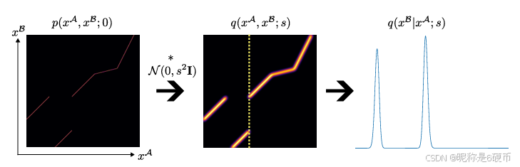
【翻译】图3. 匹配可定位性的说明。在无限分辨率下，匹配分布可以看作是一个2D表面（在图中以1D线条说明），然而在更粗糙的尺度$s$下，由于运动边界，这种分布变得模糊。这说明有必要使用能够表示多模态分布的模型和目标函数。

【解析】分辨率与匹配确定性的权衡。在理想的无限分辨率情况下，每个像素的真实匹配位置是确定的，匹配分布呈现为尖锐的峰值。然而在实际的有限分辨率下，特别是在较粗糙的尺度上，原本确定的匹配关系变得模糊不清。运动边界是指场景中不同物体或深度层之间的分界线，这些边界在投影到图像平面时产生匹配的不连续性。当分辨率降低时，这些边界附近的像素可能同时受到多个物体的影响，导致匹配分布从单峰变为多峰。传统的回归方法假设单峰分布，在面对这种多模态性时会产生平均化的预测，导致匹配精度下降。因此需要专门设计能够建模和优化多模态分布的架构和损失函数，这正是作者提出回归分类化方法的动机所在。

3.4. 鲁棒损失函数设计

Intuition: The conditional match distribution at coarse scales is more likely to exhibit multimodality than during refinement, which is conditional on the previous warp. This means that the coarse matcher needs to model multimodal distributions, which motivates our regression-byclassification approach. In contrast, the refinement of the warp needs only to represent unimodal distributions, which motivates our robust regression loss.

【翻译】直觉：粗糙尺度下的条件匹配分布比在细化过程中更容易表现出多模态性，而细化是以先前的变形为条件的。这意味着粗糙匹配器需要建模多模态分布，这促使我们采用分类回归方法。相比之下，变形的细化只需要表示单模态分布，这促使我们使用鲁棒回归损失。

【解析】（再次强调一下）粗糙匹配阶段面临的根本挑战是多模态分布问题。在粗糙尺度上，由于图像分辨率较低和运动边界的存在，同一个特征点可能对应多个候选匹配位置，形成多峰分布。这种情况下，传统的回归方法会产生平均化效应，导致预测精度下降。因此需要采用能够处理离散多选择的分类方法，将连续的匹配问题转化为在预定义锚点上的概率分布预测。细化阶段则不同，由于已经有了粗糙匹配提供的初始变形场作为先验条件，搜索空间被大幅缩小到真实匹配位置的邻域内。在这个局部邻域中，匹配分布通常呈现单峰特性，因此可以使用传统的回归方法。然而，即使在单峰情况下，如果初始估计存在较大误差，普通的$L_2$损失会产生过大的梯度，导致训练不稳定。因此采用鲁棒回归损失，在局部表现为$L_2$特性以保证精确性，在全局具有衰减梯度以提高稳定性。

Theoretical Model: We model the matchability at scale $s$ as

【翻译】理论模型：我们将尺度$s$下的可匹配性建模为：

$$q(x^A,x^B;s)=\mathcal{N}(0,s^2\mathbf{I})\ast p(x^A,x^B;0).$$

Here $p(x^A,x^B;0)$ corresponds to the exact mapping at infinite resolution. This can be interpreted as a diffusion in the localization of the matches over scales. When multiple objects in a scene are projected into images, so-called motion boundaries arise. These are discontinuities in the matches which we illustrate in Figure 3. The diffusion near these motion boundaries causes the conditional distribution to become multimodal, explaining the need for multimodality in the coarse global matching. Given an initial choice of $(x^A,x^B)$ , as in the refinement, the conditional distribution is unimodal locally. However, if this initial choice is far outside the support of the distribution, using a non-robust loss function is problematic. It is therefore motivated to use a robust regression loss for this stage.

【翻译】这里$p(x^A,x^B;0)$对应于无限分辨率下的精确映射。这可以解释为匹配在不同尺度上定位的扩散过程。当场景中的多个物体被投影到图像中时，会出现所谓的运动边界。这些是匹配中的不连续性，我们在图3中进行了说明。运动边界附近的扩散导致条件分布变为多模态，这解释了粗糙全局匹配中对多模态的需求。给定一个初始选择$(x^A,x^B)$，如在细化中，条件分布在局部是单模态的。然而，如果这个初始选择远离分布的支撑集，使用非鲁棒损失函数是有问题的。因此，在这个阶段使用鲁棒回归损失是有动机的。

【解析】这个公式描述了匹配精度随尺度变化的扩散模型。$p(x^A,x^B;0)$代表无限分辨率下的精确匹配分布，在理想情况下这是一个狄拉克函数（完全确定的点对点映射）。$\mathcal{N}(0,s^2\mathbf{I})$是方差为$s^2$的各向同性高斯核，$\ast$表示卷积操作。当尺度$s$增大时，高斯核的标准差$s$也增大，导致精确匹配分布被更大程度地平滑化。这种平滑化过程模拟了从高分辨率到低分辨率的信息损失：在低分辨率下，原本尖锐的匹配峰值变得宽泛和模糊，特别是在运动边界附近，多个物体的匹配信息混合在一起，形成多峰分布。这个理论模型解释了为什么粗糙尺度需要处理多模态分布，而细化尺度可以专注于单模态分布。

Figure 4. Comparison of loss gradients. We use the generalized Charbonnier [3] loss for refinement, which locally matches L2 gradients, but globally decays with $|x{|}^{-1/2}$ toward zero.

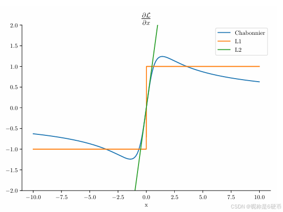
【翻译】图4. 损失梯度的比较。我们使用广义Charbonnier损失进行细化，它在局部匹配L2梯度，但在全局以$|x{|}^{-1/2}$向零衰减。

【解析】广义Charbonnier损失是一种鲁棒损失函数，它结合了$L_2$损失和$L_1$损失的优点。在误差较小的局部区域，其梯度行为类似于$L_2$损失，提供平滑的二次收敛特性，确保在接近最优解时能够快速精确地收敛。在误差较大的全局区域，梯度按$|x{|}^{-1/2}$的幂律衰减至零，这种衰减行为比$L_1$损失更加温和，避免了梯度的突然截断，同时又比$L_2$损失在大误差时更加稳健。这种设计特别适合于细化阶段的优化问题：当初始估计较为准确时，利用二次特性快速收敛到精确解；当初始估计存在较大误差时，通过梯度衰减机制避免优化过程发散，逐步引导解向正确方向移动。这种损失函数的双重特性使得细化网络既能处理高质量的粗糙匹配输入，也能对较差的初始估计保持鲁棒性。

Loss formulation: Motivated by intuition and the theoretical model we now propose our loss formulation from a probabilistic perspective, aiming to minimize the Kullback– Leibler divergence between the estimated match distribution at each scale, and the theoretical model distribution at that scale. We begin by formulating the coarse loss. With non-overlapping bins as defined in Section 3.3 the Kullback–Leibler divergence (where terms that are constant w.r.t. $\theta$ are ignored) is

$$\begin{array}{r}{D}_{\mathrm{KL}}(q(x^{\beta },x^{\mathcal{A}};s)||p_{\mathrm{coarse},\theta }(x^{\beta },x^{\mathcal{A}}))=\\ {\mathbb{E}}_{x^{\mathbf{A}},x^{\beta }\sim q}[-\log p_{\mathrm{coarse},\theta }(x^{\beta }|x^{\mathcal{A}})p_{\mathrm{coarse},\theta }(x^{\mathcal{A}})]=\\ -{\int }_{x^{\mathbf{A}},x^{\mathcal{B}}}\log {\pi }_{k^{\uparrow }}(x^{\mathbf{A}})+\log p_{\mathrm{coarse},\theta }(x^{\mathbf{A}})dq,\end{array}$$

for $k^{†}(x)={\mathrm{argmin}}_k\Vert m_k-x\Vert$ the index of the closest anchor to $x$ . Following DKM [17] we add a hyperparameter $\lambda$ that controls the weighting of the marginal compared to that of the conditional as

$$-{\int }_{x^A,x^B}\log {\pi }_{k^{†}}(x^A)+\lambda \log p_{\mathrm{coarse},\theta }(x^A)dq.$$

【翻译】损失函数制定：基于直觉和理论模型的动机，我们现在从概率的角度提出损失函数制定，旨在最小化每个尺度上估计匹配分布与该尺度理论模型分布之间的Kullback-Leibler散度。我们首先制定粗糙损失。使用第3.3节中定义的非重叠区间，Kullback-Leibler散度（忽略相对于$\theta$为常数的项）为：

其中$k^{†}(x)={\mathrm{argmin}}_k\Vert m_k-x\Vert$是距离$x$最近的锚点的索引。遵循DKM [17]，我们添加一个超参数$\lambda$来控制边际分布相对于条件分布的权重：

【解析】完整的概率损失函数。核心思想是通过最小化KL散度来让模型学习到的匹配分布$p_{\mathrm{coarse},\theta }$尽可能接近理论上的真实分布$q$。首先将联合分布分解为条件分布和边际分布的乘积，然后将连续积分转化为在离散锚点上的求和。关键的转换是$k^{†}(x)={\mathrm{argmin}}_k\Vert m_k-x\Vert$，这个函数将连续的匹配位置$x$映射到最近的离散锚点索引$k$，从而实现了从回归到分类的转换。条件项$\log p_{\mathrm{coarse},\theta }(x^{\beta }|x^{\mathcal{A}})$负责学习准确的匹配关系，而边际项$\log p_{\mathrm{coarse},\theta }(x^{\mathcal{A}})$负责学习可匹配性判断。通过调节$\lambda$，可以控制模型在匹配精度和匹配置信度之间的权衡，这对于处理遮挡、超出视野等情况下的鲁棒性至关重要。

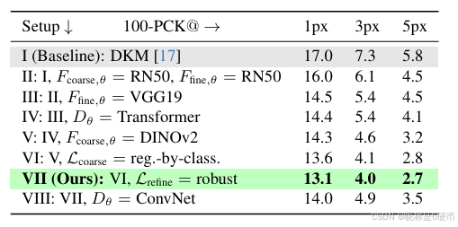
Table 2. Ablation study. We systematically investigate the impact of our contributions, see Section 4.1 for detailed analysis. Measured in 100-percentage correct keypoints (PCK) (lower is better).

【翻译】表2. 消融研究。我们系统地研究了我们贡献的影响，详细分析见第4.1节。以100-百分比正确关键点（PCK）测量（越低越好）。

In practice, we approximate $q$ with a discrete set of known correspondences {xA,xB}\{x^{A},x^{B}\}{xA,xB} . Furthermore, to be consistent with previous works [17, 52] we use a binary crossentropy loss on $p_{\mathrm{coarse},\theta }(x^A)$ . We call this loss ${\mathcal{L}}_{\mathrm{coarse}}$ . We next discuss the fine loss ${\mathcal{L}}_{\mathrm{fine}}$ .

【翻译】在实践中，我们用已知对应关系的离散集合{xA,xB}\{x^{A},x^{B}\}{xA,xB}来近似$q$。此外，为了与之前的工作[17, 52]保持一致，我们在$p_{\mathrm{coarse},\theta }(x^A)$上使用二元交叉熵损失。我们称这个损失为${\mathcal{L}}_{\mathrm{coarse}}$。接下来我们讨论细化损失${\mathcal{L}}_{\mathrm{fine}}$。

【解析】理论上我们需要真实的连续分布$q$，但实际训练时只能获得有限的已知匹配对数据集。二元交叉熵损失用于边际分布$p_{\mathrm{coarse},\theta }(x^A)$的学习，这个分布负责判断图像A中的点是否可匹配（即是否在图像B中有对应点）。这种设计使得模型能够处理遮挡、超出视野等情况，学会区分哪些点应该尝试匹配，哪些点没有有效对应关系。

We model the output of the refinement at scale $i$ as a generalized Charbonnier [3] (with $\alpha =0.5)$ distribution, for which the refiners estimate the mean $\mu$ . The generalized Charbonnier distribution behaves locally like a Normal distribution, but has a flatter tail. When used as a loss, the gradients behave locally like L2, but decay towards 0, see Figure 4. Its logarithm, (ignoring terms that do not contribute to the gradient, and up-to-scale) reads

【翻译】我们将尺度$i$下细化的输出建模为广义Charbonnier [3]分布（$\alpha =0.5$），其中细化器估计均值$\mu$。广义Charbonnier分布在局部表现得像正态分布，但具有更平坦的尾部。当用作损失时，梯度在局部表现得像L2，但衰减至0，见图4。其对数（忽略不对梯度贡献的项，且不考虑尺度）为：

【解析】广义Charbonnier分布结合了高斯分布和拉普拉斯分布的优点。参数$\alpha =0.5$控制分布的形状特性：在零点附近具有二次曲率（类似高斯分布），提供平滑的梯度用于精确收敛；在远离零点的区域，尾部比高斯分布更平坦，梯度衰减更温和，避免异常值产生过大梯度而破坏训练稳定性。细化器的任务是估计这个分布的均值$\mu$，即预测的精确匹配位置。这种建模方式使得细化过程既能在接近真实位置时快速收敛，又能在初始估计较差时保持鲁棒性。

$$\begin{array}{r}\log p_{\theta }(x_i^{\mathcal{B}}|x_i^{\mathcal{A}},{\hat{W}}_{i+1}^{\mathcal{A}\to \mathcal{B}})=\\ -(||{\mu }_{\theta }(x_i^{\mathcal{A}},{\hat{W}}_{i+1}^{\mathcal{A}\to \mathcal{B}})-x_i^{\mathcal{B}}|{|}^2+s{)}^{1/4},\end{array}$$

where ${\mu }_{\theta }(x_i^{\mathcal{A}},{\hat{W}}_{i+1}^{\mathcal{A}\to \mathcal{B}})$ is the estimated mean of the distribution, and $s=2^{i}c$ . In practice, we choose $c=0.03$ . The Kullback–Leibler divergence for each fine scale $i\in$ {0,1,2,3}\{0,1,2,3\}{0,1,2,3} (where terms that are constant with respect to $\theta$ are ignored) reads

【翻译】其中${\mu }_{\theta }(x_i^{\mathcal{A}},{\hat{W}}_{i+1}^{\mathcal{A}\to \mathcal{B}})$是分布的估计均值，$s=2^{i}c$。在实践中，我们选择$c=0.03$。每个细化尺度i∈{0,1,2,3}i\in\{0,1,2,3\}i∈{0,1,2,3}的Kullback-Leibler散度（忽略相对于$\theta$为常数的项）为：

【解析】公式是Charbonnier损失的具体形式。负对数似然中的幂指数$1/4$来源于$\alpha =0.5$的设置，这个选择在理论分析和实验验证中被证明是最优的。参数$s=2^{i}c$表示尺度相关的鲁棒性参数：在更粗糙的尺度（更大的$i$），$s$更大，损失函数对预测误差更加宽容；在更精细的尺度，$s$更小，要求更高的预测精度。常数$c=0.03$是通过实验调优得到的，它决定了鲁棒性参数的基准值，影响整个多尺度细化过程的收敛特性。

$$\begin{gathered} D_{\text{KL}}(q(x_i^B,x_i^A;s=2^{i}c)\parallel p_{i,\theta }(x_i^B,x_i^A|{\hat{W}}_{i+1}^{A\to B}))= \\ {\mathbb{E}}_{x_i^A,x_i^B\sim q}\left[-{\left({\Vert {\mu }_{\theta }(x_i^A,{\hat{W}}_{i+1}^{A\to B})-x_i^B\Vert }^2+s\right)}^{1/4}\right]+{\mathbb{E}}_{x_i^A,x_i^B\sim q}\left[-\log p_{i,\theta }(x_i^A|{\hat{W}}_{i+1}^{A\to B})\right]. \end{gathered}$$

【解析】完整的细化阶段KL散度损失函数。第一项是回归损失，通过广义Charbonnier形式惩罚预测位置${\mu }_{\theta }$与真实位置$x_i^B$之间的欧几里德距离误差。第二项是可匹配性损失，学习在给定变形场${\hat{W}}_{i+1}^{A\to B}$条件下，图像A中的点是否应该被匹配。这种双重约束确保细化网络不仅能准确预测匹配位置，还能判断哪些点值得进行细化。期望操作表示在所有训练样本上的平均，实际实现时通过批次采样来近似。

In practice, we approximate $q$ with a discrete set of known correspondences {xA,xB}\{x^{A},x^{B}\}{xA,xB} , and use a binary cross-entropy loss on $p_{\mathrm{coarse},\theta }(x_i^{\tilde{A}}|{\hat{W}}_{i+1}^{A\to \tilde{B}})$ . We sum over all fine scales to get the loss ${\mathcal{L}}_{\mathrm{fine}}$ .

【翻译】在实践中，我们用已知对应关系的离散集合{xA,xB}\{x^{A},x^{B}\}{xA,xB}来近似$q$，并在$p_{\mathrm{coarse},\theta }(x_i^{\tilde{A}}|{\hat{W}}_{i+1}^{A\to \tilde{B}})$上使用二元交叉熵损失。我们对所有细化尺度求和得到损失${\mathcal{L}}_{\mathrm{fine}}$。

【解析】实际训练细节。与粗糙阶段类似，连续分布$q$被离散的训练数据近似。二元交叉熵损失应用于条件可匹配性分布，这里的条件是给定上一级的变形场估计。多尺度求和策略使得每个细化级别都对总损失有贡献，形成从粗到细的渐进优化过程。每个尺度的损失权重隐含地通过数据分布和网络结构自动平衡，不需要人工调节尺度间的权重参数。

Our combined loss yields:

【翻译】我们的组合损失为：

$$\begin{array}{r}\mathcal{L}={\mathcal{L}}_{\mathrm{coarse}}+{\mathcal{L}}_{\mathrm{fine}}.\end{array}$$

Note that we do not need to tune any scaling between these losses as the coarse matching and fine stages are decoupled as gradients are cut in the matching, and encoders are not shared.

【翻译】注意我们不需要调节这些损失之间的任何尺度，因为粗糙匹配和细化阶段是解耦的，梯度在匹配中被截断，编码器不共享。

【解析】通过梯度截断（gradient cutting），粗糙阶段和细化阶段在训练时相互独立，避免了复杂的权重平衡问题。编码器不共享的设计进一步强化了这种解耦：粗糙编码器专注于提取适合全局匹配的鲁棒特征，细化编码器专注于提取适合局部精确定位的精细特征。

In practice, we approximate $q$ with a discrete set of known correspondences {xA,xB}\{x^{A},x^{B}\}{xA,xB} , and use a binary cross-entropy loss on $p_{\mathrm{coarse},\theta }(x_i^{\tilde{A}}|{\hat{W}}_{i+1}^{A\to \tilde{B}})$ . We sum over all fine scales to get the loss ${\mathcal{L}}_{\mathrm{fine}}$ .

【翻译】在实践中，我们用已知对应关系的离散集合{xA,xB}\{x^{A},x^{B}\}{xA,xB}来近似$q$，并在$p_{\mathrm{coarse},\theta }(x_i^{\tilde{A}}|{\hat{W}}_{i+1}^{A\to \tilde{B}})$上使用二元交叉熵损失。我们对所有细化尺度求和得到损失${\mathcal{L}}_{\mathrm{fine}}$。

Our combined loss yields:

【翻译】我们的组合损失为：

$$\begin{array}{r}\mathcal{L}={\mathcal{L}}_{\mathrm{coarse}}+{\mathcal{L}}_{\mathrm{fine}}.\end{array}$$

Note that we do not need to tune any scaling between these losses as the coarse matching and fine stages are decoupled as gradients are cut in the matching, and encoders are not shared.

【翻译】注意我们不需要调节这些损失之间的任何尺度，因为粗糙匹配和细化阶段是解耦的，梯度在匹配中被截断，编码器不共享。

4. Experiments

4.1. Ablation Study

Here we investigate the impact of our contributions. We conduct all our ablations on a validation test that we create. The validation set is made from random pairs from the MegaDepth scenes [0015, 0022] with overlap $>0$ . To measure the performance we measure the percentage of estimated matches that have an end-point-error (EPE) under a certain pixel threshold over all ground-truth correspondences, which we call percent correct keypoints (PCK) using the notation of previous work [17, 52].

【翻译】在这里我们研究我们的贡献的影响。我们在我们创建的验证测试上进行所有消融实验。验证集由来自MegaDepth场景[0015, 0022]的随机对组成，重叠度$>0$。为了衡量性能，我们测量在所有真实对应关系中，端点误差(EPE)低于某个像素阈值的估计匹配百分比，我们称之为正确关键点百分比(PCK)，使用先前工作[17, 52]的符号。

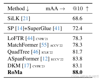
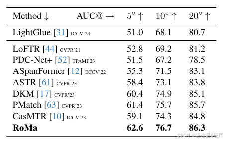
Table 3. SotA comparison on IMC2022 [25]. Measured in mAA (higher is better).

【翻译】表3. IMC2022 [25]上的最新技术比较。以mAA衡量（越高越好）。

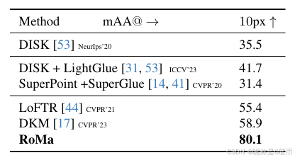
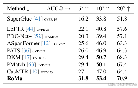
Table 4. SotA comparison on WxBS [35]. Measured in mAA at $10\mathrm{px}$ (higher is better).

【翻译】表4. WxBS [35]上的最新技术比较。以$10\mathrm{px}$处的mAA衡量（越高越好）。

Setup I consists of the same components as in DKM [17], retrained by us. In Setup II we do not share weights between the fine and coarse features, which improves performance due to specialization of the features. In Setup III we replace the RN50 fine features with a VGG19, which further improves performance. This is intriguing, as VGG19 features are worse performing when used as coarse features as we show in Table 1. We then add the proposed Transformer match decoder in Setup IV, however using the baseline regression approach. Further, we incorporate the DINOv2 coarse features in Setup V, this gives a significant improvement, owing to their significant robustness. Next, in Setup VI change the loss function and output representation of the Transformer match decoder $D_{\theta }$ to regressionby-classification, and next in Setup VII use the robust regression loss. Both these changes further significantly improve performance. This setup constitutes RoMa. When we change back to the original ConvNet match decoder in Setup VIII from this final setup, we find that the performance significantly drops, showing the importance of the proposed Transformer match decoder.

【翻译】设置I包含与DKM [17]相同的组件，由我们重新训练。在设置II中，我们不在精细和粗糙特征之间共享权重，由于特征的专业化，这提高了性能。在设置III中，我们用VGG19替换RN50精细特征，进一步提高了性能。这很有趣，因为如我们在表1中所示，当用作粗糙特征时，VGG19特征表现更差。然后我们在设置IV中添加了提出的Transformer匹配解码器，但使用基线回归方法。进一步，我们在设置V中融入DINOv2粗糙特征，由于其显著的鲁棒性，这给出了显著改进。接下来，在设置VI中，我们将Transformer匹配解码器$D_{\theta }$的损失函数和输出表示改为回归分类，然后在设置VII中使用鲁棒回归损失。这两个变化都进一步显著提高了性能。这个设置构成了RoMa。当我们从这个最终设置回到原始的ConvNet匹配解码器（设置VIII）时，我们发现性能显著下降，显示了提出的Transformer匹配解码器的重要性。

Table 5. SotA comparison on MegaDepth-1500 [28, 44]. Measured in AUC (higher is better).

【翻译】表5. MegaDepth-1500 [28, 44]上的最新技术比较。以AUC衡量（越高越好）。

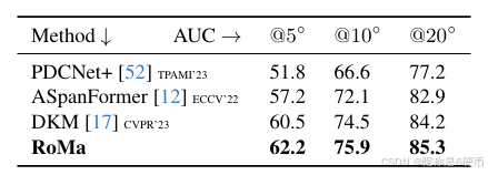
Table 6. SotA comparison on ScanNet-1500 [13, 41]. Measured in AUC (higher is better).

【翻译】表6. ScanNet-1500 [13, 41]上的最新技术比较。以AUC衡量（越高越好）。

4.2. Training Setup

We use the training setup as in DKM [17]. Following DKM, we use a canonical learning rate (for batchsize $=8\cdot$ ) of $10^{-4}$ for the decoder, and $5\cdot 10^{-6}$ for the encoder(s). We use the same training split as in DKM, which consists of randomly sampled pairs from the MegaDepth and ScanNet sets excluding the scenes used for testing. The supervised warps are derived from dense depth maps from multiview-stereo (MVS) of SfM reconstructions in the case of MegaDepth, and from RGB-D for ScanNet. Following previous work [12, 17, 44], use a model trained on the ScanNet training set when evaluating on ScanNet-1500. All other evaluation is done on a model trained only on MegaDepth.

【翻译】我们使用与DKM [17]相同的训练设置。遵循DKM，我们对解码器使用标准学习率（批大小$=8\cdot$）$10^{-4}$，对编码器使用$5\cdot 10^{-6}$。我们使用与DKM相同的训练分割，包含从MegaDepth和ScanNet集合中随机采样的对，排除用于测试的场景。对于MegaDepth，监督扭曲来自SfM重建的多视角立体(MVS)的密集深度图，对于ScanNet则来自RGB-D。遵循先前的工作[12, 17, 44]，在ScanNet-1500上评估时使用在ScanNet训练集上训练的模型。所有其他评估都是在仅在MegaDepth上训练的模型上进行的。

As in DKM we train both the coarse matching and refinement networks jointly. Note that since we detach gradients between the coarse matching and refinement, the network could in principle also be trained in two stages. For results used in the ablation, we used a resolution of $448\times 448$ , and for the final method we trained on a resolution of $560\times 560$ .

【翻译】与DKM一样，我们联合训练粗糙匹配和细化网络。注意，由于我们在粗糙匹配和细化之间分离梯度，网络原则上也可以分两阶段训练。对于消融实验中使用的结果，我们使用$448\times 448$的分辨率，对于最终方法，我们在$560\times 560$的分辨率上训练。

4.3. Two-View Geometry

We evaluate on a diverse set of two-view geometry benchmarks. We follow DKM [17] and sample correspondences using a balanced sampling approach, producing 10,000 matches, which are then used for estimation. We consistently improve compared to prior work across the board, in particular achieving a relative error reduction on the competitive IMC2022 [25] benchmark by $26\%$ , and a gain of $36\%$ in performance on the exceptionally difficult $\mathbf{WxBS}$ [35] benchmark.

【翻译】我们在多样的双视图几何基准上进行评估。我们遵循DKM [17]并使用平衡采样方法采样对应关系，产生10,000个匹配，然后用于估计。我们在各个方面都比先前工作持续改进，特别是在竞争激烈的IMC2022 [25]基准上实现了$26\%$的相对误差减少，在异常困难的$\mathbf{WxBS}$ [35]基准上获得了$36\%$的性能提升。

Table 7. SotA comparison on Megadepth-8-Scenes [17]. Measured in AUC (higher is better).

【翻译】表7. Megadepth-8-Scenes [17]上的最新技术比较。以AUC衡量（越高越好）。

Image Matching Challenge 2022: We submit to the 2022 version of the image matching challenge [25], which consists of a hidden test-set of Google street-view images with the task to estimate the fundamental matrix between them. We present results in Table 3. RoMa attains significant improvements compared to previous approaches, with a relative error reduction of $26\%$ compared to the previous best approach.

【翻译】图像匹配挑战2022：我们提交到2022版本的图像匹配挑战[25]，它包含一个隐藏的Google街景图像测试集，任务是估计它们之间的基础矩阵。我们在表3中展示结果。RoMa与先前方法相比获得了显著改进，与先前最佳方法相比相对误差减少了$26\%$。

WxBS Benchmark: We evaluate RoMa on the extremely difficult $\mathbf{WxBS}$ benchmark [35], version 1.1 with updated ground truth and evaluation protocol4. The metric is mean average precision on ground truth correspondences consistent with the estimated fundamental matrix at a 10 pixel threshold. All methods use $\mathbf{MAGSAC}++$ [2] as implemented in OpenCV. Results are presented in Table 4. Here we achieve an outstanding improvement of $36\%$ compared to the state-of-the-art. We attribute these major gains to the superior robustness of RoMa compared to previous approaches. We qualitatively present examples of this in the supplementary.

【翻译】WxBS基准：我们在极其困难的$\mathbf{WxBS}$基准[35]上评估RoMa，版本1.1具有更新的真实值和评估协议4。指标是在10像素阈值下与估计的基础矩阵一致的真实对应关系上的平均精度均值。所有方法都使用OpenCV中实现的$\mathbf{MAGSAC}++$ [2]。结果在表4中展示。在这里我们与最新技术相比实现了$36\%$的杰出改进。我们将这些重大收益归因于RoMa相比先前方法的卓越鲁棒性。我们在补充材料中定性展示了这方面的例子。

MegaDepth-1500 Pose Estimation: We use the MegaDepth-1500 test set [44] which consists of 1500 pairs from scene 0015 (St. Peter’s Basilica) and 0022 (Brandenburger Tor). We follow the protocol in [12, 44] and use a RANSAC threshold of 0.5. Results are presented in Table 5. ScanNet-1500 Pose Estimation: ScanNet [13] is a large scale indoor dataset, composed of challenging sequences with low texture regions and large changes in perspective. We follow the evaluation in SuperGlue [41]. Results are presented in Table 6. We achieve state-of-the-art results, achieving the first $AUC@20^{\circ }$ scores over 70.

【翻译】MegaDepth-1500位姿估计：我们使用MegaDepth-1500测试集[44]，它包含来自场景0015（圣彼得大教堂）和0022（勃兰登堡门）的1500对。我们遵循[12, 44]中的协议并使用0.5的RANSAC阈值。结果在表5中展示。ScanNet-1500位姿估计：ScanNet [13]是一个大规模室内数据集，由具有低纹理区域和大视角变化的挑战性序列组成。我们遵循SuperGlue [41]中的评估。结果在表6中展示。我们实现了最新技术的结果，首次实现超过70的$AUC@20^{\circ }$分数。

MegaDepth-8-Scenes: We evaluate RoMa on the Megadepth-8-Scenes benchmark [17, 28]. We present results in Table 7. Here too we outperform previous approaches.

【翻译】MegaDepth-8-Scenes：我们在Megadepth-8-Scenes基准[17, 28]上评估RoMa。我们在表7中展示结果。在这里我们也超越了先前的方法。

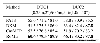
Table 8. SotA comparison on InLoc [45]. We report the percentage of query images localized within $0.25/0.5/1.0$ meters and $2/5/10^{\circ }$ of the ground-truth pose (higher is better).

【翻译】表8. InLoc [45]上的最新技术比较。我们报告在真实位姿的$0.25/0.5/1.0$米和$2/5/10^{\circ }$范围内定位的查询图像百分比（越高越好）。

4.4. Visual Localization

We evaluate RoMa on the InLoc [45] Visual Localization benchmark, using the HLoc [40] pipeline. We follow the approach in DKM [17] to sample correspondences. Results are presented in Table 8. We show large improvements compared to all previous approaches, setting a new state-of-theart.

【翻译】我们使用HLoc [40]管道在InLoc [45]视觉定位基准上评估RoMa。我们遵循DKM [17]中的方法来采样对应关系。结果在表8中展示。我们与所有先前方法相比显示出巨大改进，创立了新的最新技术水平。

4.5. Runtime Comparison

We compare the runtime of RoMa and the baseline DKM at a resolution of $560\times 560$ at a batch size of 8 on an RTX6000 GPU. We observe a modest $7\%$ increase in runtime from $186.3\to 198.8\mathrm{n}$ s per pair.

【翻译】我们在RTX6000 GPU上以$560\times 560$的分辨率和批大小为8比较了RoMa和基线DKM的运行时间。我们观察到运行时间从$186.3\to 198.8\mathrm{n}$秒每对有适度的$7\%$增加。

5. Conclusion

We have presented RoMa, a robust dense feature matcher. Our model leverages frozen pretrained coarse features from the foundation model DINOv2 together with specialized ConvNet fine features, creating a precisely localizable and robust feature pyramid. We further improved performance with our proposed tailored transformer match decoder, which predicts anchor probabilities instead of regressing coordinates. Finally, we proposed an improved loss formulation through regression-by-classification with subsequent robust regression. Our comprehensive experiments show that RoMa achieves major gains across the board, setting a new state-of-the-art. In particular, our biggest gains $36\%$ increase on WxBS [35]) are achieved on the most difficult benchmarks, highlighting the robustness of our approach. Code is provided at github.com/Parskatt/RoMa.

【翻译】我们提出了RoMa，一个鲁棒的密集特征匹配器。我们的模型利用来自基础模型DINOv2的冻结预训练粗糙特征，结合专门的ConvNet细粒度特征，创建了一个精确可定位且鲁棒的特征金字塔。我们通过提出的量身定制的transformer匹配解码器进一步改进了性能，该解码器预测锚点概率而不是回归坐标。最后，我们通过分类回归和后续鲁棒回归提出了改进的损失公式。我们的综合实验表明，RoMa在各个方面都取得了重大收益，创立了新的最新技术水平。特别是，我们最大的收益（在WxBS [35]上$36\%$的增长）是在最困难的基准上实现的，突出了我们方法的鲁棒性。代码在github.com/Parskatt/RoMa提供。

Limitations and Future Work:

(a) Our approach relies on supervised correspondences, which limits the amount of usable data. We remedied this by using pretrained frozen foundation model features, which improves generalization.

【翻译】(a) 我们的方法依赖于监督对应关系，这限制了可用数据的数量。我们通过使用预训练的冻结基础模型特征来补救这一问题，这提高了泛化能力。

(b) We train on the task of dense feature matching which is an indirect way of optimizing for the downstream tasks of two-view geometry, localization, or 3D reconstruction. Directly training on the downstream tasks could improve performance.

【翻译】(b) 我们在密集特征匹配任务上进行训练，这是优化双视图几何、定位或3D重建等下游任务的间接方式。直接在下游任务上训练可能会提高性能。