当前位置：首页 > news >正文

tinyrenderer笔记（中）

news 来源：原创 2025/5/7 6:28:48

tinyrenderer
个人代码仓库：tinyrenderer个人练习代码

前言

原教程的第 4 课与第 5 课主要介绍了坐标变换的一些知识点，但这一篇文章的内容主要是手动构建 MVP 矩阵，LookAt 矩阵以及原教程涉及到的一些知识点，不是从一个图形学小白的角度来描述。如果读者没有系统上过图形学的课程，还是建议查阅原教程，以及这篇文章：从零构建光栅器，tinyrenderer笔记（下） - 知乎。

games101：

Lecture 03 Transformation
Lecture 04 Transformation Cont

本篇使用的一切向量/矩阵规范类比 OpenGL。

齐次坐标

表示一个三维空间的点 $p$ 只需要三个分量： $(x, y, z)$ ，齐次坐标只是将 3 维扩展成了 4 维 $(x, y, z, w)$ 。这样做的主要目的是让平移操作也能用矩阵乘法实现，与其它几何变换（旋转、缩放）统一。

将齐次坐标转化为普通笛卡尔三维坐标很简单，将 $x$ 、 $y$ 、 $z$ 分量都除以 $w$ 即可： $(x / w, y / w, z / w)$ 。当 $w = 0$ 时，你会发现坐标分量无穷大，这可以代表无穷远处的点，也可以代表一个向量。

我们来模仿 OpenGl 的 glm 库，实现各种矩阵变换函数的内部细节。万丈高楼平地起，为了表示后续的矩阵，我在代码中创建了一个模板矩阵类 mat, 它位于 glm.h 下，实现了一些基本的矩阵运算：乘法、求逆、转置。

平移

有了齐次坐标之后，平移的矩阵表示非常简单：设平移向量为 $t_x, t_y, t_z)$ ，平移变换矩阵：

$\begin{bmatrix}1&0&0&t_x\\0&1&0&t_y\\0&0&1&t_z\\0&0&0&1\end{bmatrix}\begin{bmatrix}x\\y\\z\\1\end{bmatrix}=\begin{bmatrix}x+t_x\\y+t_y\\z+t_z\\1\end{bmatrix}$

glm 的 translate 函数：

translatedMatrix = glm::translate(matrix, vector);

第一个参数为要变换的矩阵，第二个参数为平移向量，这个函数的实现非常简单，不多赘述：

mat4 translate(const mat4& matrix, const Vec3f& v)
{glm::mat4 translateMatrix;for (int i = 0;i < 3;i++){translateMatrix[i][3] = v[i];}return matrix * translateMatrix;
}

缩放

设缩放因子 $s_x, s_y, s_z)$ ，缩放矩阵：

$\begin{bmatrix}s_x&0&0&0\\0&s_y&0&0\\0&0&s_z&0\\0&0&0&1\end{bmatrix}\begin{bmatrix}x\\y\\z\\1\end{bmatrix}=\begin{bmatrix}x*s_x\\y*s_y\\z*s_z\\1\end{bmatrix}$

glm 的 scale 函数：

scaledMatrix = glm::scale(matrix, vector);

模仿实现：

mat4 scale(const mat4& matrix, const Vec3f& v)
{mat4 scaleMatrix;for (int i = 0;i < 3;i++){scaleMatrix[i][i] = v[i];}return matrix * scaleMatrix;
}

旋转

三维空间下，绕任意轴 $R_x,R_y,R_z)$ 旋转 $\theta$ 的旋转矩阵要复杂许多：
$\begin{bmatrix} \cos\theta + R_x^{2}(1 - \cos\theta) & R_xR_y(1 - \cos\theta) - R_z\sin\theta & R_xR_z(1 - \cos\theta) + R_y\sin\theta & 0 \\ R_yR_x(1 - \cos\theta) + R_z\sin\theta & \cos\theta + R_y^{2}(1 - \cos\theta) & R_yR_z(1 - \cos\theta) - R_x\sin\theta & 0 \\ R_zR_x(1 - \cos\theta) - R_y\sin\theta & R_zR_y(1 - \cos\theta) + R_x\sin\theta & \cos\theta + R_z^{2}(1 - \cos\theta) & 0 \\ 0 & 0 & 0 & 1 \end{bmatrix}$

glm 的 rotate 函数：

rotatedMatrix = glm::rotate(matrix, angle, axis);

模仿实现：

mat4 rotate(const mat4& matrix, float angle, const Vec3f& axis) 
{// 将角度转换为弧度float rad = radians(angle);float cosTheta = cos(rad);float sinTheta = sin(rad);float oneMinusCos = 1.0f - cosTheta;// 归一化旋转轴Vec3f normalizedAxis = axis.normalized();float rx = normalizedAxis.x;float ry = normalizedAxis.y;float rz = normalizedAxis.z;mat4 rotateMatrix;// 第一列rotateMatrix[0][0] = cosTheta + rx * rx * oneMinusCos;rotateMatrix[0][1] = rx * ry * oneMinusCos + rz * sinTheta;rotateMatrix[0][2] = rx * rz * oneMinusCos - ry * sinTheta;// 第二列rotateMatrix[1][0] = rx * ry * oneMinusCos - rz * sinTheta;rotateMatrix[1][1] = cosTheta + ry * ry * oneMinusCos;rotateMatrix[1][2] = ry * rz * oneMinusCos + rx * sinTheta;// 第三列rotateMatrix[2][0] = rx * rz * oneMinusCos + ry * sinTheta;rotateMatrix[2][1] = ry * rz * oneMinusCos - rx * sinTheta;rotateMatrix[2][2] = cosTheta + rz * rz * oneMinusCos;return matrix * rotateMatrix;
}

模型矩阵

模型矩阵用于将物体的坐标空间从局部空间转换到世界空间下，若你还对各种坐标空间傻傻分不清楚，推荐观看 LearnOpenGL 的这篇教程：坐标系统 - LearnOpenGL CN

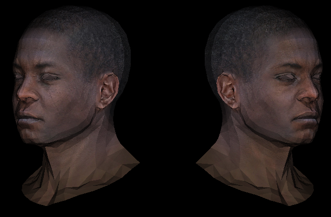
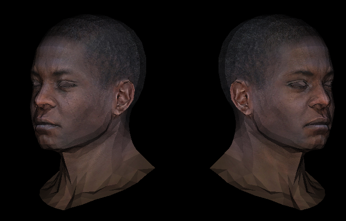
我们从 obj 文件直接读取的顶点坐标就是位于局部空间下的，之前我们只渲染了一个模型，并希望它位于屏幕的中央，所以区分局部空间与世界空间并没有多大意义。现在让我们渲染两个模型，一个在左边、一个在右边，右边的模型我们通过之前实现的变换矩阵将其缩小一倍，并且向右看，左边的同样缩小一倍，并朝左看。

首先创建一个 drawModel 函数，用于渲染特定的模型：

void drawModel(TGAImage& image, TGAImage& tex, Vec3f light_dir, float* zbuffer, Model* model, glm::mat4 modelMatrix)
{for (int i = 0; i < model->nfaces(); i++){std::vector<int> face_v = model->face_v(i);std::vector<int> face_vt = model->face_vt(i);VertexInfo vertex[3];for (int j = 0; j < 3; j++){vertex[j].textureCoor = model->textureCoor(face_vt[j]);// 得到局部空间坐标Vec3f model_coords = model->vert(face_v[j]);// 局部空间坐标转化为世界空间坐标Vec3f world_coords = modelMatrix * Vec4f(model_coords, 1.f);vertex[j].location = Vec3f((world_coords.x + 1.0) * width / 2.0, (world_coords.y + 1.0) * height / 2.0, world_coords.z);}Vec3f n = (model->vert(face_v[1]) - model->vert(face_v[0])) ^ (model->vert(face_v[2]) - model->vert(face_v[0]));n = modelMatrix.inverse().transpose().to_mat3() * n;n.normalize();float intensity = -(n * light_dir);if (intensity > 0){triangle(vertex[0], vertex[1], vertex[2], zbuffer, image, tex, intensity);}}
}

代码与之前并没有什么不同，只是多了一步，将局部空间坐标转换到世界空间，法线同样需要变换，但这里涉及到另外一个知识：法线矩阵，留到后面讲解。

在 main 函数里面：

glm::mat4 modelMatrix;
modelMatrix = glm::translate(modelMatrix, Vec3f(-0.5, 0, 0));
modelMatrix = glm::rotate(modelMatrix, 45.f, Vec3f(0, 1, 0));
modelMatrix = glm::scale(modelMatrix, Vec3f(0.5, 0.5, 0.5));
drawModel(result, texture, light_dir, zbuffer, model, modelMatrix);
modelMatrix = glm::mat4::identity();
modelMatrix = glm::translate(modelMatrix, Vec3f(0.5, 0, 0));
modelMatrix = glm::rotate(modelMatrix, -45.f, Vec3f(0, 1, 0));
modelMatrix = glm::scale(modelMatrix, Vec3f(0.5, 0.5, 0.5));
drawModel(result, texture, light_dir, zbuffer, model, modelMatrix);

结果：

视图矩阵

视图矩阵又称为观察矩阵，用于将世界空间坐标转化为视图空间（又称为摄像机空间、观察空间）坐标。在视图空间下，摄像机位于 $(0, 0, 0)$ ，并向 $(0, 0, - 1)$ 方向观察，因此视图空间就是从摄像机的视角所观察到的空间。为什么会存在这样一个坐标转换步骤呢？这其实是为了后续的投影与裁剪步骤。

三个相互垂直（或线性无关）的轴定义了一个坐标空间，我们可以利用这三个轴以及一个原点位置来构建一个变换矩阵。使用该矩阵乘以任何向量，就可以将该向量从一个坐标空间变换到新定义的坐标空间。LookAt 矩阵正是利用了这个特性。

LookAt

假设我们已经拥有了构成摄像机局部坐标系（视图空间）的三个相互垂直的轴：右向量（ $R$ ）、上向量（ $U$ ）和方向向量（ $D$ ），以及定义摄像机在世界空间中位置的 $P$ ，我们可以构建自己的 LookAt 矩阵：

$\begin{gathered}LookAt=\begin{bmatrix}R_x&R_y&R_z&0\\U_x&U_y&U_z&0\\-D_x&-D_y&-D_z&0\\0&0&0&1\end{bmatrix}*\begin{bmatrix}1&0&0&-P_x\\0&1&0&-P_y\\0&0&1&-P_z\\0&0&0&1\end{bmatrix}\end{gathered}$

其中：

$R$ ：右向量（Right Vector），表示摄像机局部坐标系的 $x$ 轴正方向。
$U$ ：上向量（Up Vector），表示摄像机局部坐标系的 $y$ 轴正方向。
$D$ ：方向向量（Direction Vector），表示摄像机局部坐标系的负 $z$ 轴方向（摄像机实际观察的方向）。
$P$ ：摄像机在世界空间中的位置（Camera Position）。

glm 的 lookAt 函数：

view = glm::lookAt(cameraPosition, targetPosition, Up);

模仿实现：

mat4 lookAt(const Vec3f& eye, const Vec3f& center, const Vec3f& up)
{Vec3f D = (center - eye).normalized();Vec3f R = D.cross(up).normalized();Vec3f U = R.cross(D);mat4 viewMatrix;viewMatrix[0][0] = R.x;viewMatrix[0][1] = R.y;viewMatrix[0][2] = R.z;viewMatrix[1][0] = U.x;viewMatrix[1][1] = U.y;viewMatrix[1][2] = U.z;viewMatrix[2][0] = -D.x;viewMatrix[2][1] = -D.y;viewMatrix[2][2] = -D.z;viewMatrix[0][3] = -R.dot(eye);viewMatrix[1][3] = -U.dot(eye);viewMatrix[2][3] = D.dot(eye);return viewMatrix;
}

假设摄像机位于 $(0, 0, - 2)$ ，并向 $(0, 0, 0)$ 看过去，则我们可以利用 lookAt 创建一个视图矩阵：

glm::mat4 viewMatrix = glm::lookAt(Vec3f(0, 0, -2), Vec3f(0, 0, 0), Vec3f(0, 1, 0));

将其传参到 drawModel 函数里，并应用起来：

// 世界空间坐标转化为视图空间坐标
Vec4f view_coords = viewMatrix * world_coords;
vertex[j].location = Vec3f((view_coords.x + 1.0) * width / 2.0, (view_coords.y + 1.0) * height / 2.0, view_coords.z);

别忘了将光照方向改为 $(0, 0, 1)$ ，让模型的背面被照亮：

Vec3f light_dir(0, 0, 1);

投影矩阵

投影矩阵会将视图空间坐标转化为裁剪空间(Clip Space)坐标，这是将 3 维空间投影到 2 维空间的关键步骤。参考这篇文章：图形学基础 - 变换 - 投影 - 知乎
投影方式分为两种：正交投影与透视投影。

正交投影

通过平行投影将物体投射到屏幕上，所有光线平行于摄像机方向，不考虑距离对物体大小的影响（即远近物体的尺寸保持一致）。

正交投影过程可概括为：

用六个参数 $(l, r, b, t, n, f)$ 定义一个 AABB 包围盒，然后将这个包围盒变换到规范视域体（OpenGL 里是 $(- 1, - 1, - 1)$ 到 $(1, 1, 1)$ ）。即从一个长方体变换到另一个定向与之相同的长方体，所以只涉及到平移和缩放操作。

第一步先将定义的包围盒移动到原点：

$\begin{pmatrix} 1 & 0 & 0 & -\frac{l+r}{2} \\ 0 & 1 & 0 & -\frac{b+t}{2} \\ 0 & 0 & 1 & -\frac{n+f}{2} \\ 0 & 0 & 0 & 1 \end{pmatrix}$

然后将包围盒各边缩放到 1：

$\begin{pmatrix} \frac{2}{r-l} & 0 & 0 & 0 \\ 0 & \frac{2}{t-b} & 0 & 0 \\ 0 & 0 & \frac{2}{n-f} & 0 \\ 0 & 0 & 0 & 1 \end{pmatrix} *\begin{pmatrix} 1 & 0 & 0 & -\frac{l+r}{2} \\ 0 & 1 & 0 & -\frac{b+t}{2} \\ 0 & 0 & 1 & -\frac{n+f}{2} \\ 0 & 0 & 0 & 1 \end{pmatrix} = \begin{pmatrix} \frac{2}{r - l} & 0 & 0 & \frac{l + r}{l - r} \\ 0 & \frac{2}{t - b} & 0 & \frac{b + t}{b - t} \\ 0 & 0 & \frac{2}{f - n} & \frac{n + f}{n - f} \\ 0 & 0 & 0 & 1 \end{pmatrix}$

注意由于摄像机朝向 $- z$ 轴，在视图空间下，所有深度值为负值，所以需要乘上一个关于 z 值的翻转矩阵：

$\begin{pmatrix} \frac{2}{r - l} & 0 & 0 & \frac{l + r}{l - r} \\ 0 & \frac{2}{t - b} & 0 & \frac{b + t}{b - t} \\ 0 & 0 & \frac{2}{f - n} & \frac{n + f}{n - f} \\ 0 & 0 & 0 & 1 \end{pmatrix} * \begin{pmatrix} 1 & 0 & 0 & 0 \\ 0 & 1 & 0 & 0 \\ 0 & 0 & -1 & 0 \\ 0 & 0 & 0 & 1 \end{pmatrix} = \begin{pmatrix} \frac{2}{r - l} & 0 & 0 & \frac{l + r}{l - r} \\ 0 & \frac{2}{t - b} & 0 & \frac{b + t}{b - t} \\ 0 & 0 & \frac{2}{n - f} & \frac{n + f}{n - f} \\ 0 & 0 & 0 & 1 \end{pmatrix}$

glm 的 ortho 函数：

glm::ortho(left, right, bottom, top, near, far);

模仿实现：

mat4 ortho(float left, float right, float bottom, float top, float n, float f)
{mat4 orthoMatrix;// 计算缩放分量orthoMatrix[0][0] = 2.0f / (right - left);orthoMatrix[1][1] = 2.0f / (top - bottom);orthoMatrix[2][2] = 2.0f / (n - f); // z轴方向反转// 计算平移分量orthoMatrix[0][3] = (left + right) / (left - right);orthoMatrix[1][3] = (bottom + top) / (bottom - top);orthoMatrix[2][3] = (n + f) / (n - f);return orthoMatrix;
}

正交投影矩阵会将顶点坐标的各分量映射到 $[- 1, 1]$ 的范围之内，而因为我们在投影矩阵中施加了 $z$ 值反转，让负的深度值变成了正的，所以这时候 $z$ 值越大代表深度值越深，更符合直觉判断了。所以我们还需要修改一下 zbuffer 的算法：

// 改成初始值为极大值
std::fill(zbuffer, zbuffer + width * height, std::numeric_limits<float>::max());
if (P.z < zbuffer[x + y * width])
{zbuffer[x + y * width] = P.z;·····
}

应用正交投影矩阵也很简单，不多赘述了：

// 将视图空间坐标转化为齐次裁剪空间坐标
Vec4f proj_coords = proMatrix * view_coords;

如果我们将正交投影矩阵定义为：

glm::mat4 projMatrix = glm::ortho(0, 1.f, -0.5, 0.5, 0.1f, 100.0f);

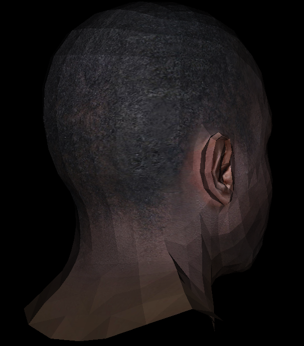
此时只会投影视图空间正 $x$ 轴部分，所以我们就只渲染出来了右边的人头：

透视投影

透视投影模拟人眼或真实摄像机的成像效果，所有光线汇聚于一点（摄像机位置），距离越远的物体在投影后显得越小（近大远小）。

透视投影矩阵的推导较为复杂，此处借鉴闫令琪老师的思想：先将视锥体“原地”变换为 AABB 包围盒，再经过平移和缩放变换到规范视域体。

所以透视投影矩阵的计算分为了两步：

第一步先将视锥体压缩为长方体
第二步将长方体经正交投影变换到规范视域体。

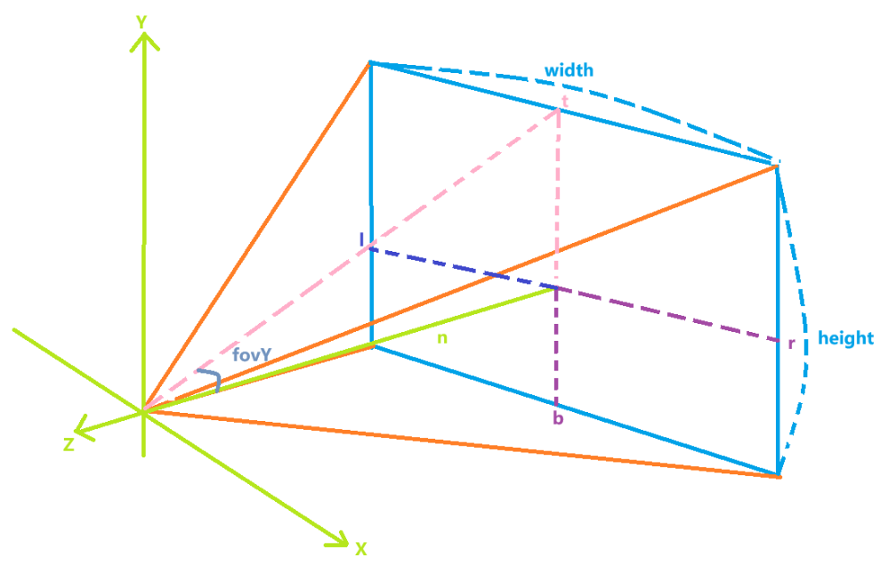
在透视投影里，视角中心穿过原点 $O$ ，设近平面宽为 $w i d t h$ ，高为 $h e i g h t$ 。设近平面左边 $x$ 坐标为 $l$ ，右边为 $r$ ，上边 $y$ 坐标为 $t$ ，下边为 $b$ ，它们满足：

$r = - l, r - l = w i d t h, t = - b, t - b = h e i g h t$

宽高比 $aspect=\frac{width}{height}=\frac{r}{t}$ ， $y$ 方向上视野角 $f o v Y$ 满足： $\frac{height}{2n}=\frac{t}{n}=\tan{\frac{fovY}{2}}$ 。

过相机位置（原点 $O$ ）作一条直线，连接三维点 $P (x, y, z, 1)$ 。这条直线与近平面相交于一点，该点即为 $P$ 在近平面上的投影 $P^\prime (x^\prime,y^\prime,z^\prime,1)$ 。根据相似三角形原理，我们可以得到以下比例关系：

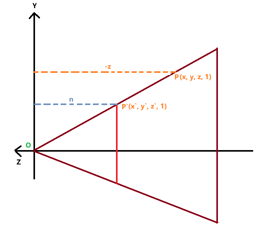
$\begin{gathered} \frac{x'}{n} = \frac{x}{-z}\\ \frac{y'}{n} = \frac{y}{-z} \end{gathered}$

通过上述比例关系，我们可以解出投影点的坐标： $x^{'} = - n x / z$ ， $y^{'} = - n y / z$ ，变换后的 $z^{'}$ 暂时未知。

因此，三维空间中的点 $(x, y, z, 1)$ 透视变换后，投影到近平面上的坐标为 $(- n x / z, - n y / z, u nkn o w n, 1)$ 。为了方便后续计算，我们将投影坐标乘以 $- z$ ，得到 $(n x, n y, u nkn o w n, - z)$ 。

根据上述投影结果，我们可以初步确定变换矩阵的形式：

$\begin{pmatrix} n & 0 & 0 & 0 \\ 0 & n & 0 & 0 \\ ? & ? & ? & ? \\ 0 & 0 & -1 & 0 \end{pmatrix} * \begin{pmatrix}x\\y\\z\\1\end{pmatrix}=\begin{pmatrix}nx\\ny\\unkonwn\\-z\end{pmatrix}$

现在需要确定变换矩阵的第三行元素。点经过透视变换后，有三点性质可以利用：

近平面上的点： $(x, y, - n, 1)$ 变换后仍位于近平面上，即 $(x, y, - n, 1)$ ，乘以 $n$ 保持不变，得到 $nx,ny,−n^2,n)$
远平面中心的点： $(0, 0, - f, 1)$ 变换后仍位于远平面中心上，即 $(0, 0, - f, 1)$ ，乘以 $f$ 保持不变，得到 $0,0,−f^2,f)$
远平面上的点： 远平面的所有点坐标 $z$ 值不变都是 $f$

我们利用第 2 点性质，可设第三行元素为： $(0, 0, A, B)$ 。又根据 1、3 条性质可得：

对于近平面点： $An+B=−n^2$
对于远平面点： $Af+B=−f^2$

联立两式，解得 $A = n + f, B = n f$ 。结合以上推导，得到第一步的结果：

$\begin{pmatrix} n & 0 & 0 & 0 \\ 0 & n & 0 & 0 \\ 0 & 0 & n+f & nf \\ 0 & 0 & -1 & 0 \end{pmatrix}$

随后就是进行一次正交投影：

$\begin{pmatrix} \frac{2}{r - l} & 0 & 0 & \frac{l + r}{l - r} \\ 0 & \frac{2}{t - b} & 0 & \frac{b + t}{b - t} \\ 0 & 0 & \frac{2}{n - f} & \frac{n + f}{n - f} \\ 0 & 0 & 0 & 1 \end{pmatrix}*\begin{pmatrix} n & 0 & 0 & 0 \\ 0 & n & 0 & 0 \\ 0 & 0 & n+f & nf \\ 0 & 0 & -1 & 0 \end{pmatrix}=\begin{pmatrix} \frac{2n}{r-l} & 0 & 0 & 0 \\ 0 & \frac{2n}{t-b} & 0 & 0 \\ 0 & 0 & \frac{n + f}{n - f} & \frac{2nf}{n - f} \\ 0 & 0 & -1 & 0 \end{pmatrix}$

请记住 $w i d t h, h e i g h t, r, l, t, b$ 是我们为了推导矩阵而定义出来的，我们只关心它们的相对关系：宽高比 $a s p ec t$ 与 $y$ 方向上的视野角 $f o v Y$ ，所以我们需要将矩阵转化一下：

$\frac{2n}{r-l}=\frac{n}{r}=\frac{n}{aspect*t}=\frac{1}{aspect*\tan{\frac{fovY}{2}}}$

$\frac{2n}{t-b}=\frac{n}{t}=\frac{1}{\tan{\frac{fovY}{2}}}$

所以最后的透视投影矩阵变为了：

$\begin{pmatrix} \frac{1}{aspect*\tan{\frac{fovY}{2}}} & 0 & 0 & 0 \\ 0 & \frac{1}{\tan{\frac{fovY}{2}}} & 0 & 0 \\ 0 & 0 & \frac{n + f}{n - f} & \frac{2nf}{n - f} \\ 0 & 0 & -1 & 0 \end{pmatrix}$

glm 的 perspective 函数：

glm::perspective(fovY, aspect, near, far);

模仿实现：

mat4 perspective(float fov, float aspect, float n, float f)
{mat4 proj;float tanHalfFov = tan(glm::radians(fov) / 2);proj[0][0] = 1 / (aspect * tanHalfFov);proj[1][1] = 1 / tanHalfFov;proj[2][2] = (f + n) / (n - f);proj[2][3] = 2 * n * f / (n - f);proj[3][2] = -1;return proj;
}

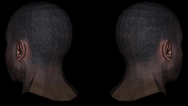
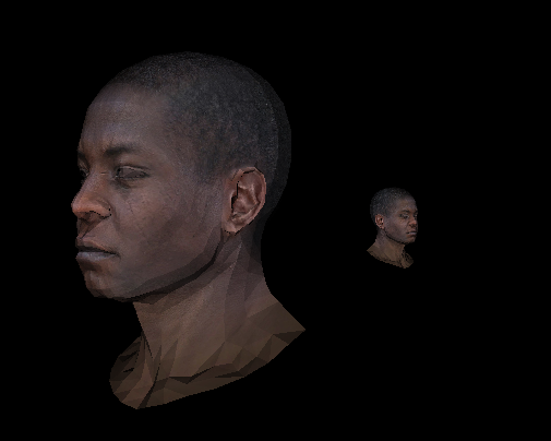
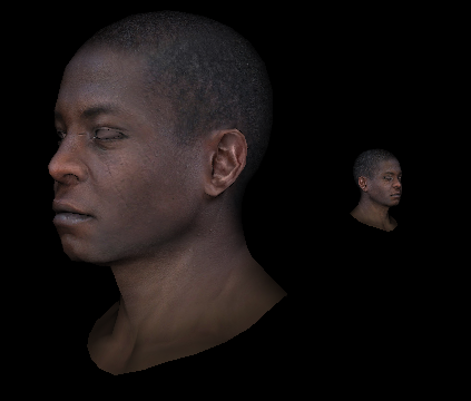
现在我们将视角换回到正面，然后将右边的模型置后，来看看近大远小的效果：

glm::mat4 projMatrix = glm::perspective(45, float(width) / height, 0.1f, 100.f);glm::mat4 modelMatrix;
modelMatrix = glm::translate(modelMatrix, Vec3f(-0.5, 0, 0));
modelMatrix = glm::rotate(modelMatrix, 45, Vec3f(0, 1, 0));
modelMatrix = glm::scale(modelMatrix, Vec3f(0.5, 0.5, 0.5));
drawModel(result, texture, light_dir, zbuffer, model, modelMatrix, viewMatrix, projMatrix);
modelMatrix = glm::mat4::identity();
modelMatrix = glm::translate(modelMatrix, Vec3f(0.5, 0, -10));
modelMatrix = glm::rotate(modelMatrix, -45, Vec3f(0, 1, 0));
modelMatrix = glm::scale(modelMatrix, Vec3f(0.5, 0.5, 0.5));
drawModel(result, texture, light_dir, zbuffer, model, modelMatrix, viewMatrix, projMatrix);

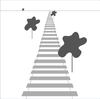
现在改为正交投影，看一下效果：

glm::mat4 projMatrix = glm::ortho(-1, 1, -1, 1, 0.1, 100);

你可以清楚地看到正交投影并没有对远处的模型进行缩放。

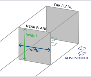
透视除法

经过透视投影矩阵变换后，坐标的各分量会处于 $[- w, w]$ 之间（正交投影 $w$ 保持不变始终为 1，所以可以不进行这一步），我们需要将其映射到 $[- 1, 1]$ 之间，这一步操作被称为透视除法，只需将各分量除以 $w$ 即可。经过透视除法后的坐标被称为 NDC（归一化/规范化设备）坐标

proj_coords = proj_coords / proj_coords.w;

这一步操作在 opengl 中是自动发生的（顶点着色器之后）。经过透视除法之后，会将坐标分量位于 $[- 1, 1]$ 之外的顶点全部剔除，不对它们进行渲染，这就是裁剪操作。

如果一个三角形三个顶点都不在 $[- 1, 1]$ 之间，那么这个三角形可以被直接裁剪。但如果这个三角形只是部分顶点不在 $[- 1, 1]$ 之内，OpenGL会重新构建这个三角形为一个或多个三角形让其能够适合这个裁剪范围。

这个重新构建三角形的算法较为复杂，现在让我们简化处理，在 triangle 函数内，不渲染那些超过范围的片段即可：

if (x < 0 || x >= width || y < 0 || y >= height){continue;}
if (P.z < -1 || P.z > 1){continue;}

视口矩阵

经过投影变换与透视除法之后，坐标都汇集到 $[- 1 ， 1]$ 的规范立方体内，然后需要经过视口变换映射到屏幕上。映射后的 $x 、 y$ 坐标范围取决于你设定的窗口大小 $\in [0,width]、y \in [0,height]$ 。映射后的深度值 $\in [0,1]$ ，当然也可以继续保持为 $[- 1, 1]$ ，我们只关心深度值的相对大小而已。

在以前的代码中，我们是这样做的：

vertex[j].location = Vec3f((proj_coords.x + 1.0) * width / 2.0, (proj_coords.y + 1.0) * height / 2.0, proj_coords.z);

这里就是视口变换，我们可以把它转化为矩阵形式：

$\begin{pmatrix} \frac{width}{2} & 0 & 0 & \frac{width}{2} \\ 0 & \frac{height}{2} & 0 & \frac{height}{2} \\ 0 & 0 & \frac{1}{2} & \frac{1}{2} \\ 0 & 0 & 0 & 1 \end{pmatrix} * \begin{pmatrix}x\\y\\z\\1\end{pmatrix}=\begin{pmatrix}\frac{(x+1)width}{2}\\\frac{(y+1)height}{2}\\\frac{z+1}{2}\\1\end{pmatrix}$

mat4 viewport(float w, float h)
{mat4 viewportMatrix;viewportMatrix[0][0] = w / 2;viewportMatrix[1][1] = h / 2;viewportMatrix[2][2] = 0.5;viewportMatrix[0][3] = w / 2;viewportMatrix[1][3] = h / 2;viewportMatrix[2][3] = 0.5;return viewportMatrix;
}

// 视口变换
Vec4f viewport_coords = viewportMatrix * proj_coords;
vertex[j].location = viewport_coords;

法线矩阵

物体表面的光照计算需要法线，而光照计算通常处于世界空间。所以我们需要将物体表面的法线从模型空间转换到世界空间下，一种简单的做法是将法线直接乘上模型矩阵，但这样做通常是错误的。请思考下面的情况（内容来自：LearnOpenGL——光照-CSDN博客，我对基础光照 - LearnOpenGL CN 的润色）：

法向量的性质： 法向量本质上是一个方向向量，它描述的是一个表面的朝向，而不是空间中的一个特定位置。与顶点位置不同，法向量没有齐次坐标中的 w 分量。这意味着平移变换不应影响法向量的方向。如果我们直接将法向量乘以一个完整的 4x4 模型矩阵，其中的平移部分会错误地影响法向量。为了消除平移的影响，我们应该只使用模型矩阵的左上角 3x3 矩阵进行变换。另一种等效的方法是将法向量的 w 分量设置为 0，然后乘以 4x4 矩阵，这样也能有效地忽略平移部分。总之，对于法向量，我们只希望应用缩放和旋转变换。
不等比缩放的影响： 更重要的是，如果模型矩阵包含不等比缩放（即在不同的轴向上缩放比例不同），那么变换后的法向量将不再垂直于变换后的表面。
- 下图展示了这种情况：
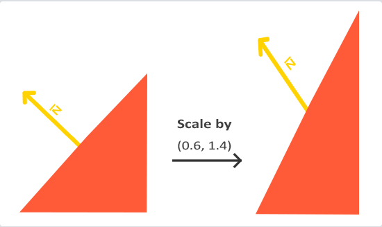
- 如图所示，原始的法向量 $N$ 垂直于表面。经过不等比缩放后，表面发生了变形，而如果直接使用模型矩阵变换法向量，得到的 $\overline{N}$ 不再垂直于新的表面。

每当我们应用一个不等比缩放时（需要注意的是，等比缩放不会破坏法线的垂直性，因为它只是改变了法线的长度，而这可以通过标准化来简单地修复），法向量就不再垂直于对应的表面，这会导致光照计算出现错误。

解决这个问题的方法是使用一个专门为法向量定制的变换矩阵，称为 法线矩阵（Normal Matrix）。法线矩阵通过特定的线性代数运算来消除不等比缩放对法向量的影响，从而保证变换后的法向量仍然垂直于变换后的表面。

如果你想知道这个矩阵是如何计算出来的，建议去阅读这个文章。译文

法线矩阵的定义是“模型矩阵左上角 3x3 部分的逆矩阵的转置矩阵”。

转置矩阵（Transpose Matrix）： 将矩阵的行和列互换得到的新矩阵。
逆矩阵（Inverse Matrix）： 一个矩阵与其逆矩阵相乘得到单位矩阵。

所以我们在 drawModel 函数内，将法线 $n$ 转换到世界空间写了如下的代码：

// 法线矩阵变换
n = modelMatrix.inverse().transpose().to_mat3() * n;
n.normalize();

Phong shading

还记得我们是如何获得三角面的法线的？我们通过三角形两边向量的叉乘来获得，这可以获得三角面宏观的法线。而三角形内部的所有着色点都是用这个宏观法线来计算光照，这就是典型的 Flat Shading 着色方法。

obj 文件内存储了三角面三个顶点的法线，我们可以将它们利用起来，内部着色点的法线可以根据重心坐标对三个顶点法线插值来得到，这样每个着色点就可以使用自己的法线来计算光照。这就是 Gouraud shading 着色方法，能带来更平滑的光照效果。

前面我们已经在 model 中存储了顶点的法线信息，现在做的工作就很简单了。先在 VertexInfo 中添加一个向量存储法线：

struct VertexInfo
{Vec3f location;Vec2f textureCoor;Vec3f normal;
};

drawModel 函数内，循环计算顶点坐标时，顺便计算一下法线信息：

for(int j = 0; j < 3; j++)
{// 法向量变换vertex[j].normal = normalMatrix * model->vertNormal(face_vn[j]);vertex[j].normal.normalize();
}

绘制三角形内部的着色点时，插值计算法线并计算光照：

Vec3f n = (t0.normal * bc_screen.x + t1.normal * bc_screen.y + t2.normal * bc_screen.z).normalize();
float light = std::max(0.f, - n * light_dir);

你可以明显地看到模型表面变光滑了！

本次代码提交记录：

这个版本的 LookAt 函数存在错误，文章是正确！2025-4-29 16.23 提交修复

Gouraud shading

原谅我在 git 的提交将 Phong shading 当作了 Gouraud shading，写完才反应过来。

理解了 Phong shading ，Gouraud shading 就很简单了。对于三角形内部的每个着色点，Gouraud shading 不是插值法线然后去计算颜色，而是直接插值三个顶点的颜色来得到内部着色点的颜色，顶点的颜色通过顶点的法线计算出来。光滑效果来说， $P h o n g > G o u r a u d > Fl a t$ 。实现很简单，就不多赘述了（其实是因为先实现了 Phong shading 而懒得实现 Gouraud shading）。