Mathematica中的ResourceFunction
在Mathematica中,ResourceFunction 的作用是访问并调用 Wolfram Function Repository(Wolfram 函数仓库)中用户或官方贡献的预定义函数。
这里给出两个使用案例:MortonCurve和LevyCCurve。
MortonCurve
和Peano曲线和Sierpinski曲线一样,MortonCurve也是一种平面填充曲线,不过填充曲线为‘Z’-型线。
ResourceFunction["MortonCurve"][n] gives the line segments representing the nth-step Morton (z-order) curve.在实际使用中,我们可以将ResourceFunction["MortonCurve"]定义为一个新的函数,然后像调用PeanoCurve一样,调用这个函数。
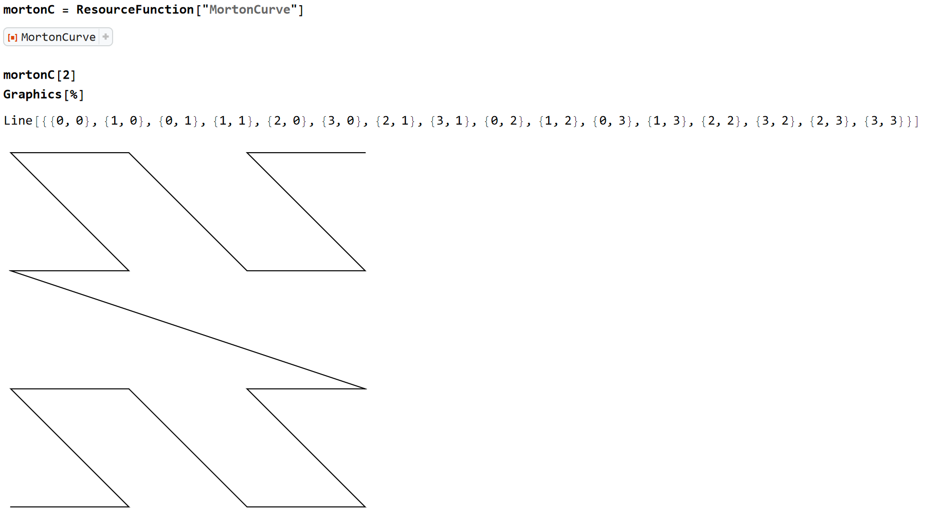
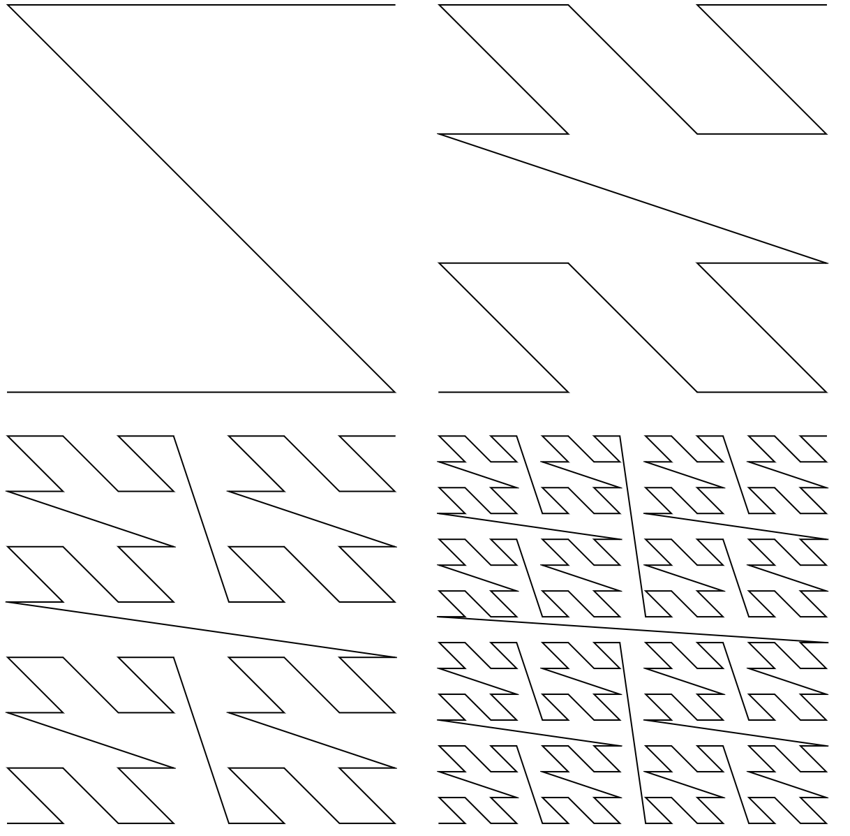
使用如下代码:
可以看到如下对比图:
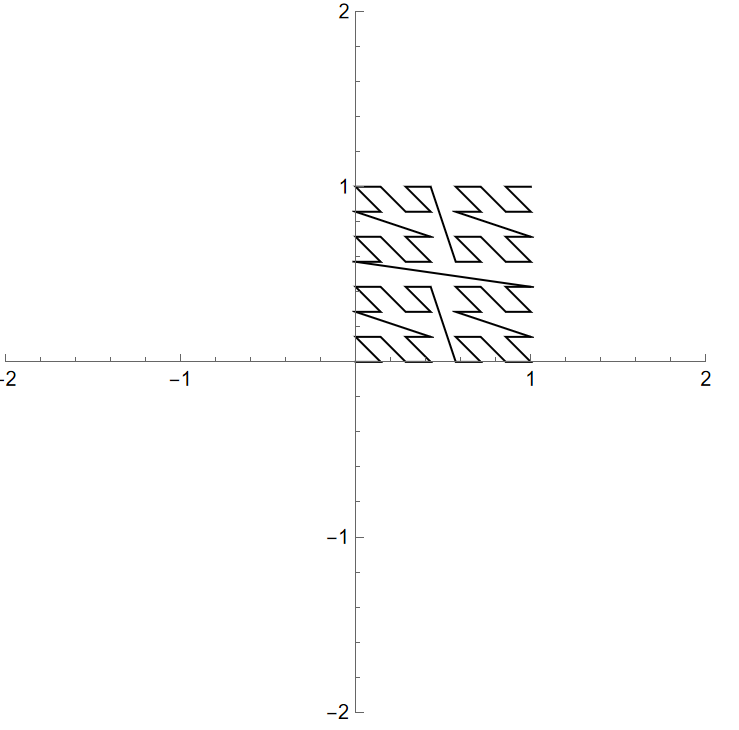
也可以指定坐标范围:
Graphics[mortonC[3, DataRange -> {{0, 1}, {0, 1}}], PlotRange -> 2, Axes -> True]
和Peano曲线一样,也可以做曲线的参数化:
BSplineFunction[mortonC[3, DataRange -> {{-1, 1}, {-1, 1}}][[1]], SplineDegree -> 1]; ParametricPlot[%[t], {t, 0, 1}, PlotPoints -> 400]
也可以使用如下方式:
Graphics[{Thickness[Large], mortonC[3] /. Line -> BSplineCurve}]

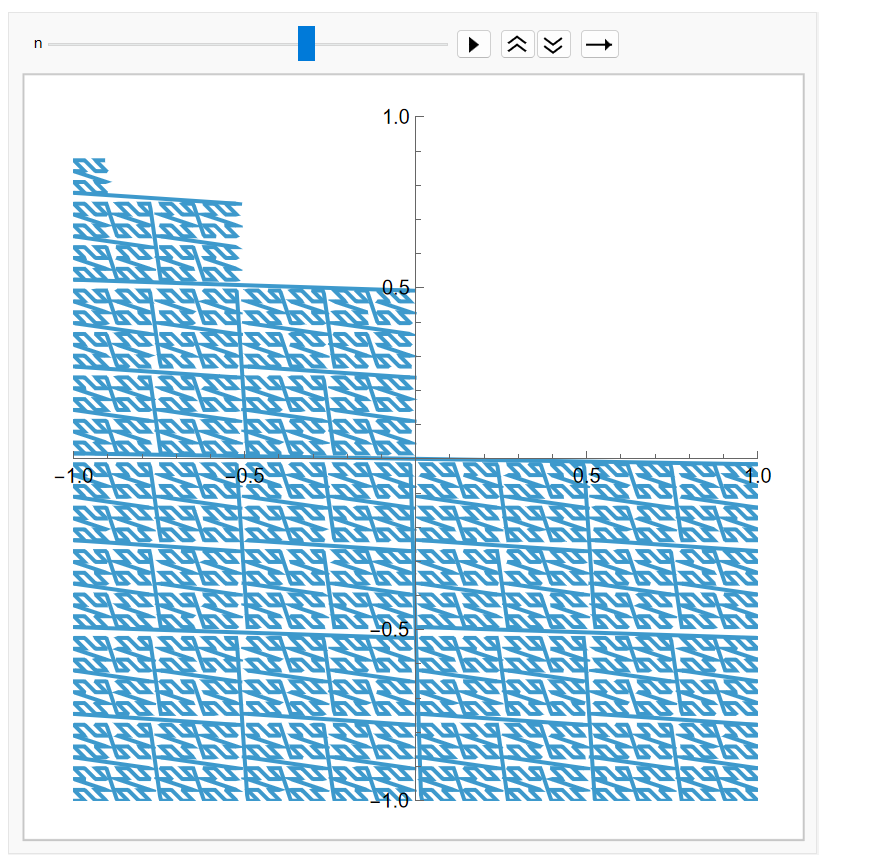
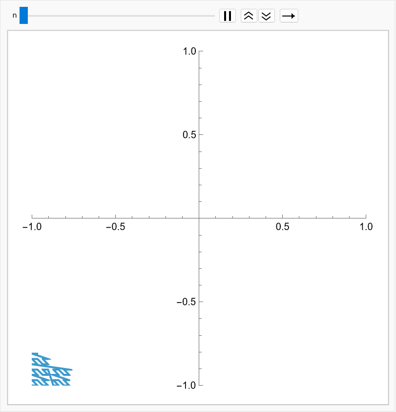
有了参数化之后,可以感测曲线的填充平面过程:
tempFunc00 = BSplineFunction[mortonC[6, DataRange -> {{-1, 1}, {-1, 1}}][[1]], SplineDegree -> 1]; Animate[ParametricPlot[tempFunc00[t], {t, 0, n}, PlotPoints -> 400, PlotRange -> {{-1, 1}, {-1, 1}}], {n, 0.01, 1, 0.01}]
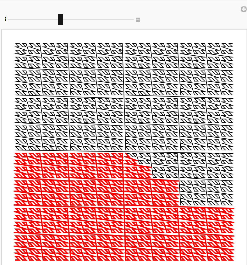
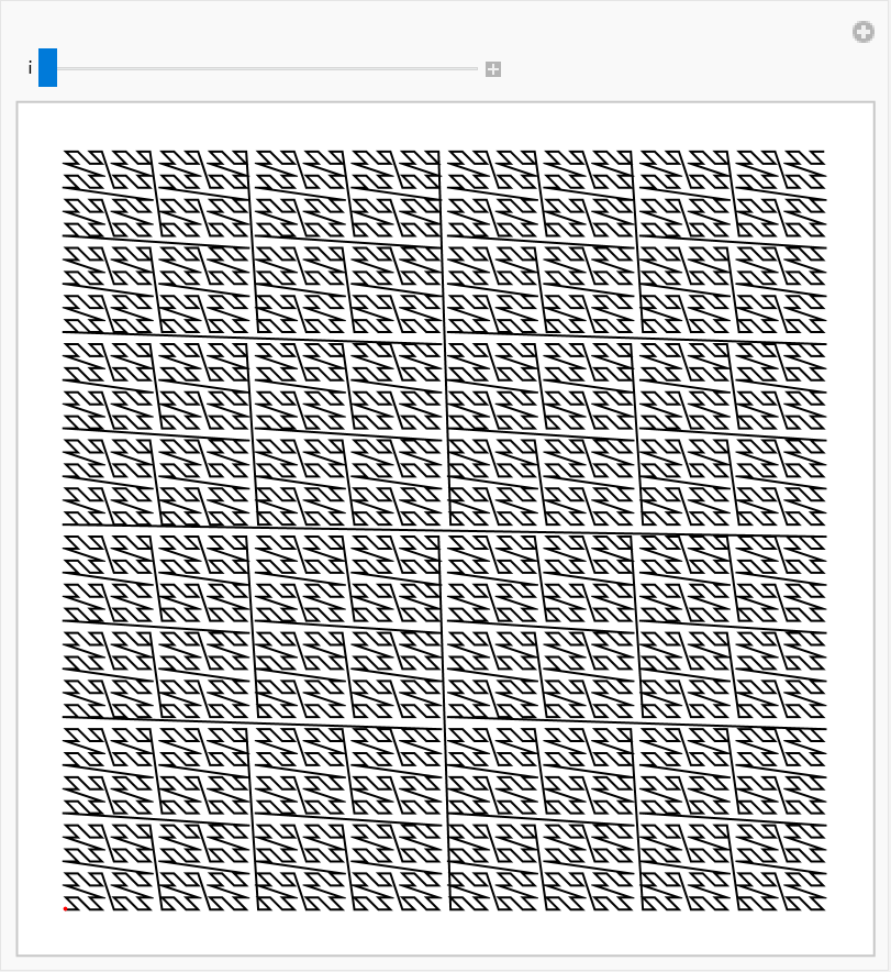
也可以使用如下方式来观察:
With[{curve = mortonC[6]}, Manipulate[ Graphics[{curve, Red, Thick, Line[Take[First[curve], i]]}, ImageSize -> Medium], {i, 1, 4096, 1}, SaveDefinitions -> True]]
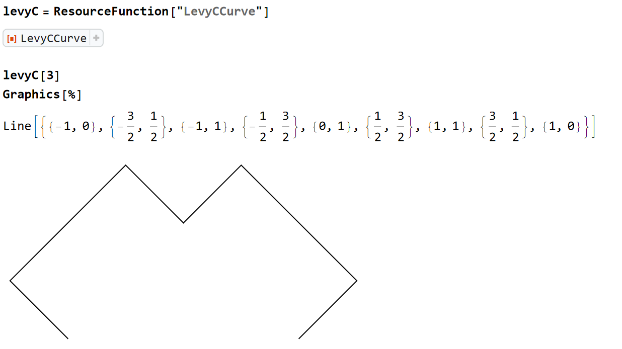
LevyCCurve
Levy C 曲线的调用语法为:
ResourceFunction["LevyCCurve"][n] generates the line segments of the Lévy C curve with n iterations. equivalent to ResourceFunction["LevyCCurve"][{{-1,0},{1,0}},n].
基本使用方法,和MortonCurve一样:
使用代码:
GraphicsGrid[ { {Graphics[levyC[2]], Graphics[levyC[3]]}, {Graphics[levyC[4]], Graphics[levyC[5]]} } ]
可以看到对比图:
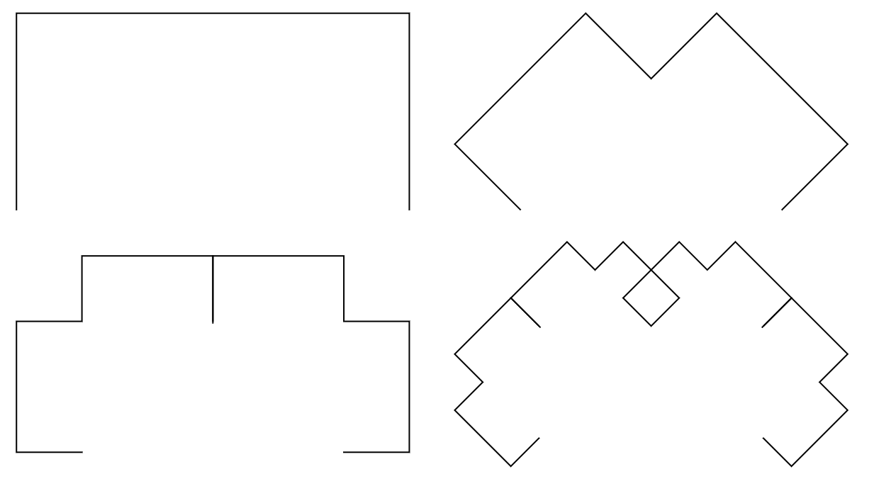
从图中可以看到:Levy C曲线,有自交。因此,不能使用BSplineFunction进行参数化。
这里提供两个比较有意思的案例,来自于官方文档的。
Graphics[{ResourceFunction["LevyCCurve"][ Line[{{0, 0}, {0, 1}, {1, 1}, {1, 0}, {0, 0}}], 10], ResourceFunction["LevyCCurve"][ Line[Reverse@{{3, 0}, {3, 1}, {4, 1}, {4, 0}, {3, 0}}], 10]}]
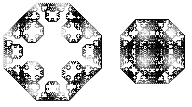
pts = First@levyC[10]; colors = Blend[{Red, Blue, Green, Orange}, #] & /@ Subdivide[Length[pts] - 1]; Graphics[Line[pts, VertexColors -> colors]]