python微分方程求解,分别用显式欧拉方法、梯形法、改进欧拉方法、二阶龙格库塔方法、四阶龙格库塔方法求解微分方程
微分方程在自然科学、工程技术、社会科学等多个领域都有着广泛而重要的应用。而求解微分方程是数学与应用数据领域一大难题,对于一些复杂的微分方程无法通过计算推导计算其精确的方程表达式与 结果,因此,我们通过数学理论。迭代,微分约等于思想寻求其精确解,随着计算机的快速发展,利用计算机程序求解微分方程非常重要,下面我们基于python代码分别利用显式欧拉方法、梯形法、改进欧拉方法、二阶龙格库塔方法、四阶龙格库塔方法求解微分方程。
1.问题描述
已知微分方程如下
其方程精确解如下:
利用python编程技术,取步长h=0.1分别1.用显示欧拉方法,2.梯形法,3.改进欧拉方法,4.二阶龙格库塔方法,5.四阶龙格库塔方法计算数值解,并于精确解比较。
2.显式欧拉方法
2.1显式欧拉方法原理
对于一阶常微分方程初值问题,
其基本思想是在每个小区间上,用差商来近似代替导数。具体来说,在
时刻,已知
,通过向前差分来近似
时刻的y值,其中h为时间步长。根据导数的定义
,将
代入可得
这就是显式欧拉方法的迭代公式,它通过已知的
和
,以及函数
来直接计算出
的值,从而逐步推进求解常微分方程在不同时刻的数值解。
2.2 python代码实现
import numpy as np
import matplotlib.pyplot as plt
# 定义微分方程
def f(x, y):
return -2 * y - 4 * x
# 定义精确解
def exact_solution(x):
return np.exp(-2 * x) - 2 * x + 1
# 显式欧拉方法
def euler_method(x0, y0, h, n):
x = np.zeros(n + 1)
y = np.zeros(n + 1)
x[0] = x0
y[0] = y0
for i in range(n):
y[i + 1] = y[i] + h * f(x[i], y[i])
x[i + 1] = x[i] + h
return x, y
# 参数设置
x0 = 0
y0 = 2
h = 0.1
n = int(1 / h)
# 计算数值解
x_euler, y_euler = euler_method(x0, y0, h, n)
# 计算精确解
x_exact = np.linspace(x0, x0 + 1, n + 1)
y_exact = exact_solution(x_exact)
# 打印结果并绘图比较
print("显式欧拉方法结果:", y_euler)
plt.plot(x_exact, y_exact, label='Exact Solution')
plt.plot(x_euler, y_euler, 'o-', label='Euler Method')
plt.xlabel('x')
plt.ylabel('y')
plt.title('Numerical Solutions Comparison')
plt.legend()
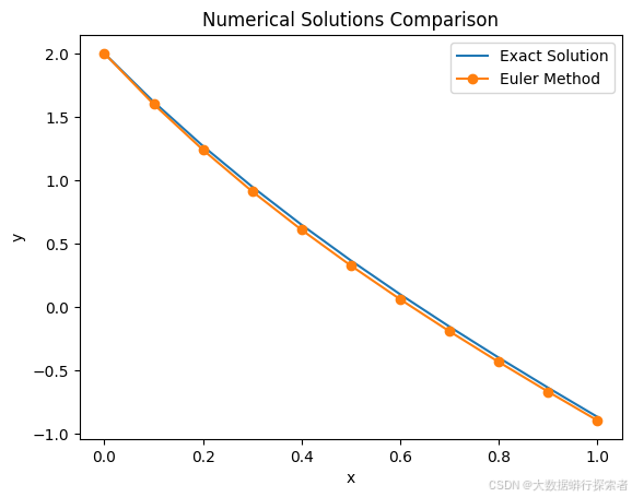
plt.show()运行结果
3.梯形法
3.1梯形法原理
考虑一阶常微分方程的初值问题:,
其中
是已知的函数,
和
分别是初始时刻和初始条件。在数值求解过程中,我们将时间区间进行离散化,设时间步长为 h,
。
显式欧拉方法是基于向前差分近似导数得到
,它仅使用了当前时刻
的斜率
。
而梯形法结合了当前时刻 和下一时刻
的斜率信息。根据积分中值定理,
梯形法使用梯形公式来近似这个积分,即。
由此得到梯形法的迭代公式:
与显式欧拉方法不同,梯形法的迭代公式是隐式的,因为 同时出现在等式的两边。这意味着在每一步求解
时,通常需要求解一个非线性方程。
3.2 python代码实现
import numpy as np
import matplotlib.pyplot as plt

# 定义微分方程
def f(x, y):
    return -2 * y - 4 * x

# 定义精确解
def exact_solution(x):
    return np.exp(-2 * x) - 2 * x + 1

# 梯形法
def trapezoid_method(f, x0, y0, h, n):
    x_values = [x0]
    y_values = [y0]
    x = x0
    y = y0
    for _ in range(n):
        def g(y_next):
            return y_next - y - 0.5 * h * (f(x, y) + f(x + h, y_next))
        from scipy.optimize import root
        sol = root(g, y)
        y = sol.x[0]
        x = x + h
        x_values.append(x)
        y_values.append(y)
    return x_values, y_values
# 参数设置
x0 = 0
y0 = 2
h = 0.1
n = int(1 / h)

# 计算数值解
x_trapezoid, y_trapezoid = trapezoid_method(f, x0, y0, h, n)
# 计算精确解
x_exact = np.linspace(x0, x0 + 1, n + 1)
y_exact = exact_solution(x_exact)

# 打印结果并绘图比较
print("梯形方法结果:", y_trapezoid)
plt.plot(x_exact, y_exact, label='Exact Solution')
plt.plot(x_trapezoid, y_trapezoid, 'o-', label='Trapezoid Method')
plt.xlabel('x')
plt.ylabel('y')
plt.title('Numerical Solutions Comparison')
plt.legend()
plt.show()
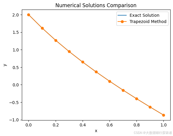
运行结果
4.改进欧拉方法
4.1改进欧拉方法原理
改进欧拉方法的核心思想是综合考虑当前点和预测的下一个点\
处的斜率信息,通过取二者的平均值作为这一步的平均斜率,以此来得到更准确的
的估计值。
具体原理和步骤
改进欧拉方法采用了预测 - 校正的策略,具体步骤如下:
- 预测阶段 利用显式欧拉方法对
时刻的y值进行初步预测。设时间步长为h,
,预测公式为:
这里
是对
的一个初步估计,它基于当前点
处的斜率
得到。
- 校正阶段 计算
时刻的斜率
,然后取这两个斜率的平均值作为这一步的平均斜率,再用这个平均斜率来校正
的值。校正公式为:
从几何角度看,改进欧拉方法不再仅仅依赖于当前点的斜率,而是综合考虑了当前点和预测点的斜率,用这两个斜率的平均值来确定在区间
上的近似直线的斜率,从而使近似曲线更接近真实的解曲线。
4.2 python代码实现
import numpy as np
import matplotlib.pyplot as plt

# 定义微分方程
def f(x, y):
    return -2 * y - 4 * x

# 定义精确解
def exact_solution(x):
    return np.exp(-2 * x) - 2 * x + 1

# 改进的欧拉方法
def improved_euler_method(x0, y0, h, n):
    x = np.zeros(n + 1)
    y = np.zeros(n + 1)
    x[0] = x0
    y[0] = y0
    for i in range(n):
        k1 = f(x[i], y[i])
        k2 = f(x[i] + h, y[i] + h * k1)
        y[i + 1] = y[i] + h * (k1 + k2) / 2
        x[i + 1] = x[i] + h
    return x, y
# 参数设置
x0 = 0
y0 = 2
h = 0.1
n = int(1 / h)

# 计算数值解
x_euler, y_euler =improved_euler_method(x0, y0, h, n)
# 计算精确解
x_exact = np.linspace(x0, x0 + 1, n + 1)
y_exact = exact_solution(x_exact)

# 打印结果并绘图比较
print("改进的欧拉方法:", y_euler)
plt.plot(x_exact, y_exact, label='Exact Solution')
plt.plot(x_euler, y_euler, 'o-', label='Improved Euler Method')
plt.xlabel('x')
plt.ylabel('y')
plt.title('Numerical Solutions Comparison')
plt.legend()
plt.show()
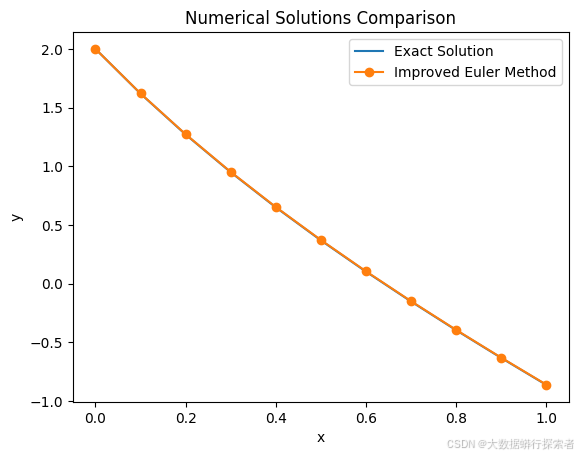
运行结果
5.二阶龙格库塔方法
5.1二阶龙格库塔方法原理
二阶龙格 - 库塔方法的基本思想是在每个时间步长内,通过计算两个不同点的斜率估计值,然后对这些斜率进行加权平均,以此来得到更准确的\(y_{n + 1}\)的估计值。
二阶龙格 - 库塔方法的一般形式可以表示为:
其中、
、
和
是待确定的参数,需要满足一定的条件以保证方法具有二阶精度。
5.2 python代码实现
import numpy as np
import matplotlib.pyplot as plt

# 定义微分方程
def f(x, y):
    return -2 * y - 4 * x

# 定义精确解
def exact_solution(x):
    return np.exp(-2 * x) - 2 * x + 1

# 二阶龙格-库塔方法
def second_order_rk_method(x0, y0, h, n):
    x = np.zeros(n + 1)
    y = np.zeros(n + 1)
    x[0] = x0
    y[0] = y0
    for i in range(n):
        k1 = h * f(x[i], y[i])
        k2 = h * f(x[i] + h / 2, y[i] + k1 / 2)
        y[i + 1] = y[i] + k2
        x[i + 1] = x[i] + h
    return x, y
# 计算精确解
x_exact = np.linspace(x0, x0 + 1, n + 1)
y_exact = exact_solution(x_exact)
x_second_order_rk, y_second_order_rk = second_order_rk_method(x0, y0, h, n)
# 参数设置
x0 = 0
y0 = 2
h = 0.1
n = int(1 / h)
plt.plot(x_exact, y_exact, label='Exact Solution')
plt.plot(x_second_order_rk, y_second_order_rk, '^-', label='Second Order RK Method')
plt.xlabel('x')
plt.ylabel('y')
plt.title('Numerical Solutions Comparison')
plt.legend()
plt.show()
运行结果

6.四阶龙格库塔方法
6.1四阶龙格库塔方法原理
前面提到的显式欧拉方法仅使用当前点的斜率来估计下一个点的值,精度较低;二阶龙格 - 库塔方法通过计算两个不同点的斜率估计值并加权平均来提高精度。四阶龙格 - 库塔方法进一步拓展了这一思想,在每个时间步长内计算四个不同点的斜率估计值,然后对这些斜率进行加权平均,从而得到更准确的的估计值。
四阶龙格 - 库塔方法公式
给定时间步长h,从到
,四阶龙格 - 库塔方法的更新公式如下:
- 计算
:
- 这里
处的斜率乘以步长h,它反映了从当前点出发的初始斜率信息。
- 这里
- 计算
:
和预测的函数值
处的斜率乘以步长h。通过在时间区间的中点进行斜率估计,考虑了函数在该区间内的变化趋势。
- 计算
:
,进一步细化了对区间内斜率的估计。
- 计算
:
处的斜率乘以步长h,反映了在该时间步结束时的斜率信息。
- 更新
- 最终的
、
、
- 最终的
6.2 python代码实现
import numpy as np
import matplotlib.pyplot as plt

# 定义微分方程
def f(x, y):
    return -2 * y - 4 * x

# 定义精确解
def exact_solution(x):
    return np.exp(-2 * x) - 2 * x + 1

# 四阶龙格-库塔方法
def fourth_order_rk_method(x0, y0, h, n):
    x = np.zeros(n + 1)
    y = np.zeros(n + 1)
    x[0] = x0
    y[0] = y0
    for i in range(n):
        k1 = h * f(x[i], y[i])
        k2 = h * f(x[i] + h / 2, y[i] + k1 / 2)
        k3 = h * f(x[i] + h / 2, y[i] + k2 / 2)
        k4 = h * f(x[i] + h, y[i] + k3)
        y[i + 1] = y[i] + (k1 + 2 * k2 + 2 * k3 + k4) / 6
        x[i + 1] = x[i] + h
    return x, y

# 计算精确解
x_exact = np.linspace(x0, x0 + 1, n + 1)
y_exact = exact_solution(x_exact)
x_fourth_order_rk, y_fourth_order_rk = fourth_order_rk_method(x0, y0, h, n)
# 参数设置
x0 = 0
y0 = 2
h = 0.1
n = int(1 / h)
plt.plot(x_exact, y_exact, label='Exact Solution')
plt.plot(x_fourth_order_rk, y_fourth_order_rk,'s-', label='Fourth Order RK Method')
plt.xlabel('x')
plt.ylabel('y')
plt.title('Numerical Solutions Comparison')
plt.legend()
plt.show()
运行结果

7.总结
为了直观的比较以上5种方法计算的准确性,将5种计算结果统一绘图比较分析。
import numpy as np
import matplotlib.pyplot as plt

# 定义微分方程
def f(x, y):
    return -2 * y - 4 * x

# 定义精确解
def exact_solution(x):
    return np.exp(-2 * x) - 2 * x + 1

# 显式欧拉方法
def euler_method(x0, y0, h, n):
    x = np.zeros(n + 1)
    y = np.zeros(n + 1)
    x[0] = x0
    y[0] = y0
    for i in range(n):
        y[i + 1] = y[i] + h * f(x[i], y[i])
        x[i + 1] = x[i] + h
    return x, y
# 梯形法
def trapezoid_method(f, x0, y0, h, n):
    x_values = [x0]
    y_values = [y0]
    x = x0
    y = y0
    for _ in range(n):
        def g(y_next):
            return y_next - y - 0.5 * h * (f(x, y) + f(x + h, y_next))
        from scipy.optimize import root
        sol = root(g, y)
        y = sol.x[0]
        x = x + h
        x_values.append(x)
        y_values.append(y)
    return x_values, y_values

# 改进的欧拉方法
def improved_euler_method(x0, y0, h, n):
    x = np.zeros(n + 1)
    y = np.zeros(n + 1)
    x[0] = x0
    y[0] = y0
    for i in range(n):
        k1 = f(x[i], y[i])
        k2 = f(x[i] + h, y[i] + h * k1)
        y[i + 1] = y[i] + h * (k1 + k2) / 2
        x[i + 1] = x[i] + h
    return x, y

# 二阶龙格-库塔方法
def second_order_rk_method(x0, y0, h, n):
    x = np.zeros(n + 1)
    y = np.zeros(n + 1)
    x[0] = x0
    y[0] = y0
    for i in range(n):
        k1 = h * f(x[i], y[i])
        k2 = h * f(x[i] + h / 2, y[i] + k1 / 2)
        y[i + 1] = y[i] + k2
        x[i + 1] = x[i] + h
    return x, y

# 四阶龙格-库塔方法
def fourth_order_rk_method(x0, y0, h, n):
    x = np.zeros(n + 1)
    y = np.zeros(n + 1)
    x[0] = x0
    y[0] = y0
    for i in range(n):
        k1 = h * f(x[i], y[i])
        k2 = h * f(x[i] + h / 2, y[i] + k1 / 2)
        k3 = h * f(x[i] + h / 2, y[i] + k2 / 2)
        k4 = h * f(x[i] + h, y[i] + k3)
        y[i + 1] = y[i] + (k1 + 2 * k2 + 2 * k3 + k4) / 6
        x[i + 1] = x[i] + h
    return x, y

# 参数设置
x0 = 0
y0 = 2
h = 0.1
n = int(1 / h)

# 计算数值解
x_euler, y_euler = euler_method(x0, y0, h, n)
x_improved_euler, y_improved_euler = improved_euler_method(x0, y0, h, n)
x_second_order_rk, y_second_order_rk = second_order_rk_method(x0, y0, h, n)
x_fourth_order_rk, y_fourth_order_rk = fourth_order_rk_method(x0, y0, h,n)
x_trapezoid, y_trapezoid = trapezoid_method(f, x0, y0, h, n)

# 计算精确解
x_exact = np.linspace(x0, x0 + 1, n + 1)
y_exact = exact_solution(x_exact)

# 打印结果并绘图比较
print("显式欧拉方法结果:", y_euler)
print("改进的欧拉方法结果:", y_improved_euler)
print("二阶龙格-库塔方法结果:", y_second_order_rk)
print("四阶龙格-库塔方法结果:", y_fourth_order_rk)
print("精确解结果:", y_exact)

plt.plot(x_exact, y_exact, label='Exact Solution')
plt.plot(x_euler, y_euler, 'o-', label='Euler Method')
plt.plot(x_improved_euler, y_improved_euler, 'x-', label='Improved Euler Method')
plt.plot(x_second_order_rk, y_second_order_rk, '^-', label='Second Order RK Method')
plt.plot(x_fourth_order_rk, y_fourth_order_rk,'s-', label='Fourth Order RK Method')
plt.plot(x_trapezoid, y_trapezoid, '*-', label='Trapezoid Method')
plt.xlabel('x')
plt.ylabel('y')
plt.title('Numerical Solutions Comparison')
plt.legend()
plt.show()
运行结果
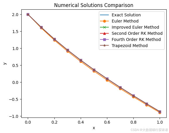
对比五种计算方法结果相差较小, 二阶龙格库塔方法计算结果最精确,