当前位置：首页 > news >正文

数据分析综合应用实战：从统计分析到机器学习预测

news 2025/10/28 9:14:25

数据分析是将原始数据转化为有价值信息的过程，涉及数据清洗、统计分析、可视化以及机器学习预测等多个环节。本文将通过三个完整的实战案例，带你掌握数据分析的全流程。

1. 豆瓣电影Top250统计分析

数据获取与清洗

首先我们需要获取豆瓣电影Top250的数据，并进行必要的数据清洗：

import pandas as pd
import numpy as np
import matplotlib.pyplot as plt
import seaborn as sns
from sklearn.linear_model import LinearRegression
from sklearn.model_selection import train_test_split
from sklearn.metrics import mean_squared_error, r2_score
import warnings
warnings.filterwarnings('ignore')# 设置中文字体
plt.rcParams['font.sans-serif'] = ['SimHei']
plt.rcParams['axes.unicode_minus'] = False# 模拟创建豆瓣电影Top250数据集
def create_douban_data():"""创建模拟的豆瓣电影Top250数据集"""np.random.seed(42)data = []movies = ['肖申克的救赎', '霸王别姬', '阿甘正传', '这个杀手不太冷', '泰坦尼克号','千与千寻', '美丽人生', '海上钢琴师', '辛德勒的名单', '盗梦空间','忠犬八公的故事', '星际穿越', '楚门的世界', '三傻大闹宝莱坞', '放牛班的春天','大话西游', '熔炉', '教父', '当幸福来敲门', '龙猫']for i in range(250):movie_id = i % len(movies)rating = np.random.normal(9.0, 0.3)rating = max(8.0, min(9.5, rating))  # 限制在8.0-9.5之间votes = np.random.randint(500000, 2000000)year = np.random.randint(1950, 2023)# 添加一些缺失值if i % 50 == 0:rating = np.nandata.append({'排名': i + 1,'电影名称': f"{movies[movie_id]}_{i}",'评分': rating,'评价人数': votes,'年份': year,'地区': np.random.choice(['美国', '中国', '日本', '韩国', '法国', '英国'], p=[0.4, 0.2, 0.15, 0.1, 0.1, 0.05])})return pd.DataFrame(data)# 创建数据集
df_douban = create_douban_data()
print("豆瓣电影Top250数据集概览:")
print(df_douban.head())
print(f"\n数据集形状: {df_douban.shape}")

output:

   排名       电影名称        评分     评价人数    年份  地区
0   1   肖申克的救赎_0       NaN   759178  2021  中国
1   2     霸王别姬_1  8.958521  1603462  1973  日本
2   3     阿甘正传_2  9.023950   827069  1987  美国
3   4  这个杀手不太冷_3  8.952145   603355  1970  日本
4   5    泰坦尼克号_4  9.006667  1933257  2009  美国数据集形状: (250, 6)

数据质量检测与处理

def data_quality_analysis(df):"""数据质量分析"""print("=== 数据质量分析 ===")# 检测缺失值missing_data = df.isnull().sum()print("缺失值统计:")print(missing_data)# 可视化缺失值plt.figure(figsize=(10, 6))plt.subplot(1, 2, 1)sns.heatmap(df.isnull(), cbar=True, cmap='viridis')plt.title('缺失值热力图')plt.subplot(1, 2, 2)missing_data.plot(kind='bar')plt.title('各列缺失值数量')plt.xticks(rotation=45)plt.tight_layout()plt.show()return missing_data# 执行数据质量分析
missing_info = data_quality_analysis(df_douban)# 处理缺失值
def handle_missing_data(df):"""处理缺失数据"""df_clean = df.copy()# 用中位数填充评分缺失值rating_median = df_clean['评分'].median()df_clean['评分'] = df_clean['评分'].fillna(rating_median)print(f"用中位数({rating_median:.2f})填充评分缺失值")print(f"填充后缺失值数量: {df_clean.isnull().sum().sum()}")return df_cleandf_cleaned = handle_missing_data(df_douban)

output:

=== 数据质量分析 ===
缺失值统计:
排名      0
电影名称    0
评分      5
评价人数    0
年份      0
地区      0
dtype: int64

统计分析

def statistical_analysis(df):"""进行统计分析"""print("=== 统计分析 ===")# 基本统计信息print("数值列基本统计:")print(df[['评分', '评价人数', '年份']].describe())# 按评分排序df_sorted_by_rating = df.sort_values('评分', ascending=False)print(f"\n评分最高的5部电影:")print(df_sorted_by_rating[['电影名称', '评分', '年份']].head())# 按评价人数排序df_sorted_by_votes = df.sort_values('评价人数', ascending=False)print(f"\n评价人数最多的5部电影:")print(df_sorted_by_votes[['电影名称', '评价人数', '评分']].head())# 各地区电影数量统计region_counts = df['地区'].value_counts()print(f"\n各地区电影数量:")print(region_counts)# 评分相关性分析correlation = df[['评分', '评价人数', '年份']].corr()print(f"\n数值特征相关性矩阵:")print(correlation)return df_sorted_by_rating, df_sorted_by_votes, correlationdf_rating_sorted, df_votes_sorted, corr_matrix = statistical_analysis(df_cleaned)

output:

=== 统计分析 ===
数值列基本统计:评分          评价人数           年份
count  245.000000  2.500000e+02   250.000000
mean     8.992839  1.233330e+06  1985.780000
std      0.279989  4.364475e+05    21.704746
min      8.177714  5.010620e+05  1950.000000
25%      8.808829  8.571668e+05  1965.250000
50%      9.013682  1.206388e+06  1987.000000
75%      9.172967  1.631638e+06  2006.000000
max      9.500000  1.974271e+06  2022.000000评分最高的5部电影:电影名称   评分    年份
249     盗梦空间_249  9.5  2011
207    海上钢琴师_207  9.5  1987
90    忠犬八公的故事_90  9.5  1959
73    三傻大闹宝莱坞_73  9.5  1964
113  三傻大闹宝莱坞_113  9.5  2007评价人数最多的5部电影:电影名称     评价人数        评分
105    千与千寻_105  1974271  9.114840
8      辛德勒的名单_8  1965689  8.391984
135    大话西游_135  1965585  9.442998
194  放牛班的春天_194  1950976  8.302094
169    盗梦空间_169  1948021  9.172852各地区电影数量:
美国    98
中国    53
日本    33
韩国    32
法国    26
英国     8
Name: 地区, dtype: int64数值特征相关性矩阵:评分      评价人数        年份
评分    1.000000 -0.014487  0.058167
评价人数 -0.014487  1.000000  0.001758
年份    0.058167  0.001758  1.000000

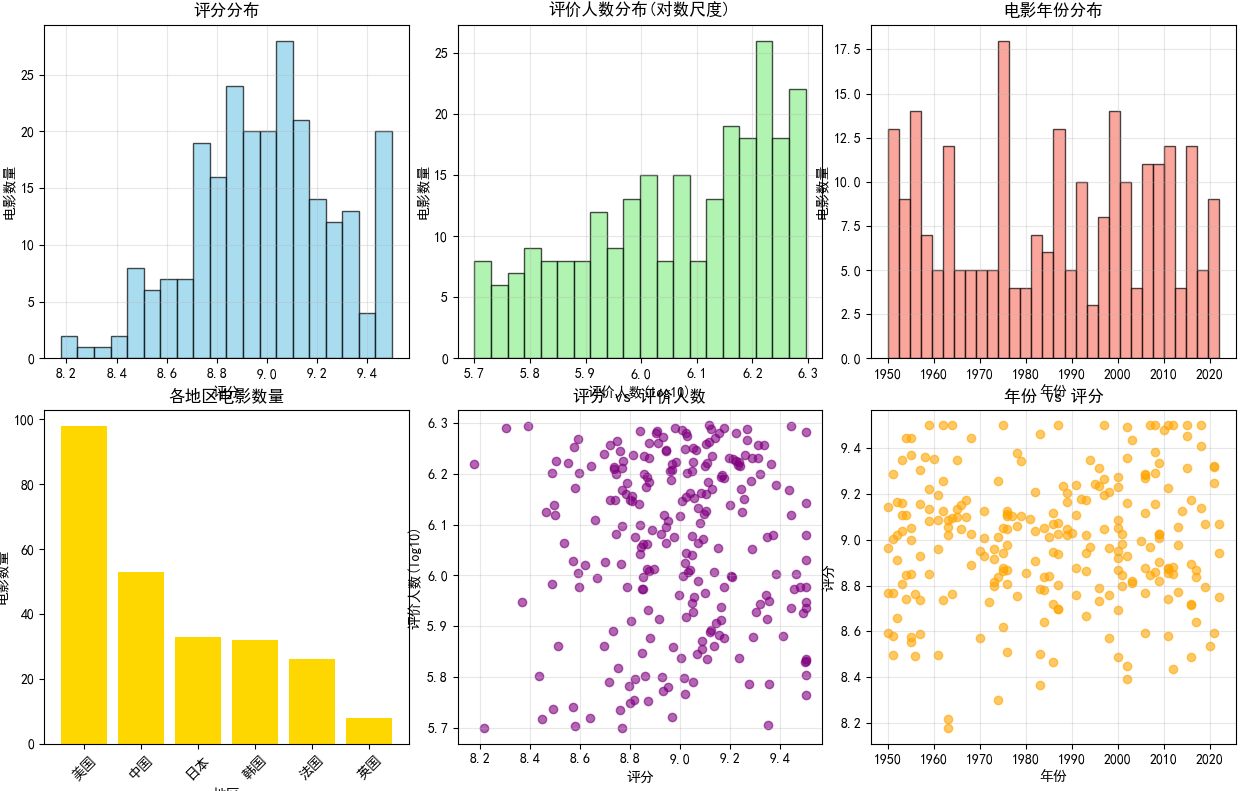
数据可视化

def douban_visualization(df):"""豆瓣数据可视化"""print("=== 数据可视化 ===")fig, axes = plt.subplots(2, 3, figsize=(18, 12))# 1. 评分分布直方图axes[0, 0].hist(df['评分'], bins=20, alpha=0.7, color='skyblue', edgecolor='black')axes[0, 0].set_xlabel('评分')axes[0, 0].set_ylabel('电影数量')axes[0, 0].set_title('评分分布')axes[0, 0].grid(True, alpha=0.3)# 2. 评价人数分布（取对数）axes[0, 1].hist(np.log10(df['评价人数']), bins=20, alpha=0.7, color='lightgreen', edgecolor='black')axes[0, 1].set_xlabel('评价人数(log10)')axes[0, 1].set_ylabel('电影数量')axes[0, 1].set_title('评价人数分布(对数尺度)')axes[0, 1].grid(True, alpha=0.3)# 3. 年份分布axes[0, 2].hist(df['年份'], bins=30, alpha=0.7, color='salmon', edgecolor='black')axes[0, 2].set_xlabel('年份')axes[0, 2].set_ylabel('电影数量')axes[0, 2].set_title('电影年份分布')axes[0, 2].grid(True, alpha=0.3)# 4. 各地区电影数量region_counts = df['地区'].value_counts()axes[1, 0].bar(region_counts.index, region_counts.values, color='gold')axes[1, 0].set_xlabel('地区')axes[1, 0].set_ylabel('电影数量')axes[1, 0].set_title('各地区电影数量')axes[1, 0].tick_params(axis='x', rotation=45)# 5. 评分与评价人数散点图axes[1, 1].scatter(df['评分'], np.log10(df['评价人数']), alpha=0.6, color='purple')axes[1, 1].set_xlabel('评分')axes[1, 1].set_ylabel('评价人数(log10)')axes[1, 1].set_title('评分 vs 评价人数')axes[1, 1].grid(True, alpha=0.3)# 6. 评分与年份关系axes[1, 2].scatter(df['年份'], df['评分'], alpha=0.6, color='orange')axes[1, 2].set_xlabel('年份')axes[1, 2].set_ylabel('评分')axes[1, 2].set_title('年份 vs 评分')axes[1, 2].grid(True, alpha=0.3)plt.tight_layout()plt.show()# 相关性热力图plt.figure(figsize=(8, 6))numeric_cols = ['评分', '评价人数', '年份']sns.heatmap(df[numeric_cols].corr(), annot=True, cmap='coolwarm', center=0)plt.title('特征相关性热力图')plt.show()# 执行可视化
douban_visualization(df_cleaned)

在这里插入图片描述

2. 在线用户时区分析

数据准备与处理

def create_user_timezone_data():"""创建模拟的用户时区数据"""np.random.seed(123)# 定义时区分布（模拟真实世界的分布）timezones = ['America/New_York', 'America/Los_Angeles', 'Europe/London', 'Europe/Paris', 'Asia/Shanghai', 'Asia/Tokyo', 'Australia/Sydney', 'Asia/Kolkata', 'America/Chicago','Europe/Moscow', 'Asia/Singapore', 'America/Toronto','Europe/Berlin', 'Asia/Dubai', 'Brazil/East','Africa/Cairo', 'Asia/Seoul', 'Pacific/Auckland','Unknown', ''  # 添加一些未知和空值时区]# 设置不同时区的概率权重weights = [15, 12, 8, 7, 20, 6, 4, 8, 5, 3, 4, 3, 5, 2, 2, 1, 2, 1, 1, 1]n_users = 10000user_data = []for i in range(n_users):timezone = np.random.choice(timezones, p=np.array(weights)/sum(weights))user_data.append({'user_id': f'user_{i:05d}','timezone': timezone,'activity_level': np.random.choice(['高', '中', '低'], p=[0.2, 0.5, 0.3])})return pd.DataFrame(user_data)# 创建用户时区数据
df_users = create_user_timezone_data()
print("用户时区数据概览:")
print(df_users.head())
print(f"\n总用户数: {len(df_users)}")

时区统计分析

def timezone_analysis(df):"""时区数据分析"""print("=== 时区数据分析 ===")# 检查缺失数据missing_timezones = df['timezone'].isnull() | (df['timezone'] == '')print(f"缺失或空值时区数量: {missing_timezones.sum()}")# 处理缺失值df_clean = df[~missing_timezones].copy()print(f"清洗后用户数量: {len(df_clean)}")# 统计各时区用户数量timezone_counts = df_clean['timezone'].value_counts()print(f"\n总时区数量: {len(timezone_counts)}")# 获取Top10时区top10_timezones = timezone_counts.head(10)print("\nTop10时区用户分布:")for tz, count in top10_timezones.items():percentage = (count / len(df_clean)) * 100print(f"{tz}: {count}人 ({percentage:.1f}%)")return df_clean, timezone_counts, top10_timezonesdf_clean_users, timezone_counts, top10_timezones = timezone_analysis(df_users)

时区数据可视化

def timezone_visualization(timezone_counts, top10_timezones):"""时区数据可视化"""print("=== 时区数据可视化 ===")fig, axes = plt.subplots(2, 2, figsize=(16, 12))# 1. Top10时区水平条形图axes[0, 0].barh(range(len(top10_timezones)), top10_timezones.values, color='lightblue')axes[0, 0].set_yticks(range(len(top10_timezones)))axes[0, 0].set_yticklabels(top10_timezones.index)axes[0, 0].set_xlabel('用户数量')axes[0, 0].set_title('Top10时区用户分布')axes[0, 0].grid(True, alpha=0.3)# 2. 时区分布饼图（Top10 + 其他）top10_sum = top10_timezones.sum()other_sum = timezone_counts.sum() - top10_sumpie_data = list(top10_timezones.values) + [other_sum]pie_labels = list(top10_timezones.index) + ['其他时区']axes[0, 1].pie(pie_data, labels=pie_labels, autopct='%1.1f%%', startangle=90)axes[0, 1].set_title('时区分布饼图')# 3. 所有时区分布折线图axes[1, 0].plot(range(len(timezone_counts)), timezone_counts.values, marker='o', linewidth=2, markersize=4)axes[1, 0].set_xlabel('时区排名')axes[1, 0].set_ylabel('用户数量')axes[1, 0].set_title('时区用户数量分布')axes[1, 0].grid(True, alpha=0.3)axes[1, 0].set_yscale('log')  # 使用对数坐标# 4. 累积分布图cumulative_counts = timezone_counts.cumsum()axes[1, 1].plot(range(len(cumulative_counts)), cumulative_counts.values, color='red', linewidth=2)axes[1, 1].set_xlabel('时区数量')axes[1, 1].set_ylabel('累积用户数量')axes[1, 1].set_title('时区用户累积分布')axes[1, 1].grid(True, alpha=0.3)# 添加一些统计信息axes[1, 1].text(0.6, 0.3, f'Top10时区覆盖用户: {top10_sum/len(df_clean_users)*100:.1f}%', transform=axes[1, 1].transAxes, fontsize=12,bbox=dict(boxstyle="round,pad=0.3", facecolor="lightyellow"))plt.tight_layout()plt.show()# 使用pandas内置绘图plt.figure(figsize=(12, 6))top10_timezones.plot(kind='barh', color='lightgreen')plt.title('Top10时区用户分布 (Pandas绘图)')plt.xlabel('用户数量')plt.tight_layout()plt.show()# 执行时区可视化
timezone_visualization(timezone_counts, top10_timezones)

3. 机器学习回归预测：波士顿房价

数据准备与探索

from sklearn.datasets import fetch_california_housing
from sklearn.preprocessing import StandardScaler
from sklearn.linear_model import LinearRegression, Ridge, Lasso
from sklearn.ensemble import RandomForestRegressor
from sklearn.svm import SVRdef load_and_explore_data():"""加载和探索数据集"""# 使用加利福尼亚房价数据集（波士顿房价数据集已弃用）print("=== 加州房价数据集分析 ===")housing = fetch_california_housing()# 创建DataFramedf_housing = pd.DataFrame(housing.data, columns=housing.feature_names)df_housing['Price'] = housing.targetprint("数据集基本信息:")print(f"数据集形状: {df_housing.shape}")print(f"特征数量: {len(housing.feature_names)}")print(f"样本数量: {len(df_housing)}")print("\n特征名称:")for i, feature in enumerate(housing.feature_names):print(f"{i+1}. {feature}")print("\n数据集前5行:")print(df_housing.head())print("\n基本统计信息:")print(df_housing.describe())# 检查缺失值print(f"\n缺失值统计:")print(df_housing.isnull().sum())return df_housing, housingdf_housing, housing_dataset = load_and_explore_data()

output:

=== 加州房价数据集分析 ===
数据集基本信息:
数据集形状: (20640, 9)
特征数量: 8
样本数量: 20640特征名称:
1. MedInc
2. HouseAge
3. AveRooms
4. AveBedrms
5. Population
6. AveOccup
7. Latitude
8. Longitude数据集前5行:MedInc  HouseAge  AveRooms  AveBedrms  ...  AveOccup  Latitude  Longitude  Price
0  8.3252      41.0  6.984127   1.023810  ...  2.555556     37.88    -122.23  4.526
1  8.3014      21.0  6.238137   0.971880  ...  2.109842     37.86    -122.22  3.585
2  7.2574      52.0  8.288136   1.073446  ...  2.802260     37.85    -122.24  3.521
3  5.6431      52.0  5.817352   1.073059  ...  2.547945     37.85    -122.25  3.413
4  3.8462      52.0  6.281853   1.081081  ...  2.181467     37.85    -122.25  3.422[5 rows x 9 columns]基本统计信息:MedInc      HouseAge  ...     Longitude         Price
count  20640.000000  20640.000000  ...  20640.000000  20640.000000
mean       3.870671     28.639486  ...   -119.569704      2.068558
std        1.899822     12.585558  ...      2.003532      1.153956
min        0.499900      1.000000  ...   -124.350000      0.149990
25%        2.563400     18.000000  ...   -121.800000      1.196000
50%        3.534800     29.000000  ...   -118.490000      1.797000
75%        4.743250     37.000000  ...   -118.010000      2.647250
max       15.000100     52.000000  ...   -114.310000      5.000010[8 rows x 9 columns]缺失值统计:
MedInc        0
HouseAge      0
AveRooms      0
AveBedrms     0
Population    0
AveOccup      0
Latitude      0
Longitude     0
Price         0
dtype: int64

数据预处理与特征工程

def preprocess_data(df):"""数据预处理和特征工程"""print("=== 数据预处理 ===")# 分离特征和目标变量X = df.drop('Price', axis=1)y = df['Price']# 数据标准化scaler = StandardScaler()X_scaled = scaler.fit_transform(X)print("数据标准化完成")print(f"标准化后数据形状: {X_scaled.shape}")# 划分训练集和测试集X_train, X_test, y_train, y_test = train_test_split(X_scaled, y, test_size=0.3, random_state=42)print(f"训练集大小: {X_train.shape}")print(f"测试集大小: {X_test.shape}")return X_train, X_test, y_train, y_test, scalerX_train, X_test, y_train, y_test, scaler = preprocess_data(df_housing)

模型训练与评估

def train_and_evaluate_models(X_train, X_test, y_train, y_test):"""训练和评估多个回归模型"""print("=== 模型训练与评估 ===")models = {'线性回归': LinearRegression(),'岭回归': Ridge(alpha=1.0),'Lasso回归': Lasso(alpha=0.1),'随机森林': RandomForestRegressor(n_estimators=100, random_state=42),'支持向量机': SVR(kernel='rbf', C=1.0)}results = {}for name, model in models.items():print(f"\n训练 {name}...")# 训练模型model.fit(X_train, y_train)# 预测y_pred = model.predict(X_test)# 评估指标mse = mean_squared_error(y_test, y_pred)r2 = r2_score(y_test, y_pred)mae = np.mean(np.abs(y_test - y_pred))results[name] = {'model': model,'mse': mse,'r2': r2,'mae': mae,'predictions': y_pred}print(f"{name} 性能:")print(f"  均方误差(MSE): {mse:.4f}")print(f"  R²分数: {r2:.4f}")print(f"  平均绝对误差(MAE): {mae:.4f}")return results# 训练和评估模型
model_results = train_and_evaluate_models(X_train, X_test, y_train, y_test)

模型结果可视化与分析

def visualize_model_results(results, y_test):"""可视化模型结果"""print("=== 模型结果可视化 ===")fig, axes = plt.subplots(2, 2, figsize=(16, 12))# 1. 模型性能比较model_names = list(results.keys())mse_scores = [results[name]['mse'] for name in model_names]r2_scores = [results[name]['r2'] for name in model_names]x_pos = np.arange(len(model_names))axes[0, 0].bar(x_pos - 0.2, mse_scores, 0.4, label='MSE', alpha=0.7, color='red')axes[0, 0].set_ylabel('均方误差(MSE)')axes[0, 0].set_title('模型MSE比较')axes[0, 0].set_xticks(x_pos)axes[0, 0].set_xticklabels(model_names, rotation=45)axes[0, 0].legend()axes[0, 0].grid(True, alpha=0.3)ax2 = axes[0, 0].twinx()ax2.bar(x_pos + 0.2, r2_scores, 0.4, label='R²', alpha=0.7, color='blue')ax2.set_ylabel('R²分数')ax2.legend(loc='upper right')# 2. 预测值与真实值散点图（最佳模型）best_model_name = max(results.keys(), key=lambda x: results[x]['r2'])best_predictions = results[best_model_name]['predictions']axes[0, 1].scatter(y_test, best_predictions, alpha=0.6, color='green')axes[0, 1].plot([y_test.min(), y_test.max()], [y_test.min(), y_test.max()], 'r--', lw=2)axes[0, 1].set_xlabel('真实价格')axes[0, 1].set_ylabel('预测价格')axes[0, 1].set_title(f'{best_model_name} - 预测vs真实值')axes[0, 1].grid(True, alpha=0.3)# 添加R²到图中r2_best = results[best_model_name]['r2']axes[0, 1].text(0.05, 0.95, f'R² = {r2_best:.4f}', transform=axes[0, 1].transAxes,bbox=dict(boxstyle="round,pad=0.3", facecolor="white"))# 3. 残差图residuals = y_test - best_predictionsaxes[1, 0].scatter(best_predictions, residuals, alpha=0.6, color='orange')axes[1, 0].axhline(y=0, color='red', linestyle='--')axes[1, 0].set_xlabel('预测价格')axes[1, 0].set_ylabel('残差')axes[1, 0].set_title(f'{best_model_name} - 残差图')axes[1, 0].grid(True, alpha=0.3)# 4. 误差分布axes[1, 1].hist(residuals, bins=30, alpha=0.7, color='purple', edgecolor='black')axes[1, 1].set_xlabel('残差')axes[1, 1].set_ylabel('频率')axes[1, 1].set_title(f'{best_model_name} - 残差分布')axes[1, 1].grid(True, alpha=0.3)# 添加正态分布曲线from scipy.stats import normmu, std = norm.fit(residuals)xmin, xmax = axes[1, 1].get_xlim()x = np.linspace(xmin, xmax, 100)p = norm.pdf(x, mu, std)axes[1, 1].plot(x, p, 'k', linewidth=2)plt.tight_layout()plt.show()return best_model_namebest_model = visualize_model_results(model_results, y_test)
print(f"\n最佳模型: {best_model}")

特征重要性分析

def analyze_feature_importance(results, housing_dataset, feature_names):"""分析特征重要性"""print("=== 特征重要性分析 ===")# 获取随机森林模型（如果存在）if '随机森林' in results:rf_model = results['随机森林']['model']# 特征重要性importance = rf_model.feature_importances_feature_importance = pd.DataFrame({'feature': feature_names,'importance': importance}).sort_values('importance', ascending=False)print("特征重要性排序:")for i, row in feature_importance.iterrows():print(f"{row['feature']}: {row['importance']:.4f}")# 可视化特征重要性plt.figure(figsize=(10, 6))plt.barh(feature_importance['feature'], feature_importance['importance'], color='teal')plt.xlabel('特征重要性')plt.title('随机森林特征重要性')plt.gca().invert_yaxis()plt.grid(True, alpha=0.3)plt.tight_layout()plt.show()# 线性模型系数分析if '线性回归' in results:lr_model = results['线性回归']['model']coefficients = pd.DataFrame({'feature': feature_names,'coefficient': lr_model.coef_}).sort_values('coefficient', key=abs, ascending=False)print("\n线性回归系数（按绝对值排序）:")for i, row in coefficients.iterrows():print(f"{row['feature']}: {row['coefficient']:.4f}")# 可视化系数plt.figure(figsize=(10, 6))colors = ['red' if x < 0 else 'blue' for x in coefficients['coefficient']]plt.barh(coefficients['feature'], coefficients['coefficient'], color=colors)plt.xlabel('系数值')plt.title('线性回归系数')plt.axvline(x=0, color='black', linestyle='-', alpha=0.3)plt.grid(True, alpha=0.3)plt.tight_layout()plt.show()# 分析特征重要性
analyze_feature_importance(model_results, housing_dataset, housing_dataset.feature_names)

4. 性能评估指标详解

def explain_evaluation_metrics(y_true, y_pred):"""详细解释回归评估指标"""print("=== 回归评估指标详解 ===")# 计算各种指标mse = mean_squared_error(y_true, y_pred)rmse = np.sqrt(mse)mae = np.mean(np.abs(y_true - y_pred))r2 = r2_score(y_true, y_pred)# 手动计算R²ss_res = np.sum((y_true - y_pred) ** 2)ss_tot = np.sum((y_true - np.mean(y_true)) ** 2)r2_manual = 1 - (ss_res / ss_tot)print(f"均方误差 (MSE): {mse:.4f}")print(f"  解释: 预测误差的平方的平均值，对异常值敏感")print(f"根均方误差 (RMSE): {rmse:.4f}")print(f"  解释: MSE的平方根，与目标变量同单位")print(f"平均绝对误差 (MAE): {mae:.4f}")print(f"  解释: 预测误差的绝对值的平均值，对异常值不敏感")print(f"R²分数: {r2:.4f} (手动计算: {r2_manual:.4f})")print(f"  解释: 模型解释的方差比例，1为完美拟合，0为均值模型")# 可视化不同指标的含义plt.figure(figsize=(12, 4))# MAE可视化plt.subplot(1, 3, 1)errors = np.abs(y_true - y_pred)plt.hist(errors, bins=30, alpha=0.7, color='blue', edgecolor='black')plt.axvline(mae, color='red', linestyle='--', linewidth=2, label=f'MAE = {mae:.2f}')plt.xlabel('绝对误差')plt.ylabel('频率')plt.title('MAE - 平均绝对误差')plt.legend()plt.grid(True, alpha=0.3)# MSE可视化plt.subplot(1, 3, 2)squared_errors = (y_true - y_pred) ** 2plt.hist(squared_errors, bins=30, alpha=0.7, color='green', edgecolor='black')plt.axvline(mse, color='red', linestyle='--', linewidth=2, label=f'MSE = {mse:.2f}')plt.xlabel('平方误差')plt.ylabel('频率')plt.title('MSE - 均方误差')plt.legend()plt.grid(True, alpha=0.3)# R²可视化plt.subplot(1, 3, 3)y_mean = np.mean(y_true)total_variation = np.sum((y_true - y_mean) ** 2)explained_variation = np.sum((y_pred - y_mean) ** 2)unexplained_variation = np.sum((y_true - y_pred) ** 2)variations = [explained_variation, unexplained_variation]labels = ['解释的方差', '未解释的方差']colors = ['lightblue', 'lightcoral']plt.pie(variations, labels=labels, colors=colors, autopct='%1.1f%%', startangle=90)plt.title(f'R² = {r2:.3f}\n(解释的方差比例)')plt.tight_layout()plt.show()# 使用最佳模型的预测结果来解释指标
best_predictions = model_results[best_model]['predictions']
explain_evaluation_metrics(y_test, best_predictions)

5. 完整数据分析管道

def complete_data_analysis_pipeline():"""完整的数据分析管道"""print("=== 完整数据分析管道 ===")# 1. 数据收集与清洗print("步骤1: 数据收集与清洗")df_douban = create_douban_data()df_cleaned = handle_missing_data(df_douban)# 2. 探索性数据分析print("步骤2: 探索性数据分析")statistical_analysis(df_cleaned)douban_visualization(df_cleaned)# 3. 机器学习建模print("步骤3: 机器学习建模")df_housing, housing_dataset = load_and_explore_data()X_train, X_test, y_train, y_test, scaler = preprocess_data(df_housing)results = train_and_evaluate_models(X_train, X_test, y_train, y_test)# 4. 模型评估与优化print("步骤4: 模型评估与优化")best_model = visualize_model_results(results, y_test)analyze_feature_importance(results, housing_dataset, housing_dataset.feature_names)# 5. 结果解释与报告print("步骤5: 结果解释与报告")explain_evaluation_metrics(y_test, results[best_model]['predictions'])print("\n完整数据分析管道执行完毕！")# 执行完整管道
complete_data_analysis_pipeline()