BEVFUSION解读（八）

激光雷达点云处理方法

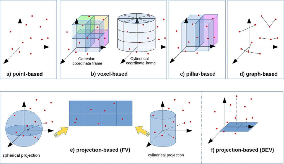
展示了多种处理雷达点云数据的方法，每种方法根据不同的坐标表示、分辨率和结构特点来处理数据。以下是每种方法的简介：

1. 点基方法 (Point-based) (a)

   • 点云数据直接表示为散布在三维空间中的点。每个点都有其在空间中的位置（x, y, z 坐标）。这种方法非常基础，适用于处理原始的雷达点云数据，但缺乏结构化的表示，处理效率较低，尤其是在大规模点云数据时。

2. 体素基方法 (Voxel-based) (b)

   • 该方法将三维空间划分为体素（类似于三维网格），每个体素包含一定数量的点。通过对点云进行体素化处理，可以将不规则的点云转换为规则的网格结构。这种方法适用于提高处理效率，尤其在使用卷积神经网络（CNN）时效果较好。图中展示了以笛卡尔坐标系和圆柱坐标系两种方式进行体素划分。

3. 柱基方法 (Pillar-based) (c)

   • 柱基方法是将点云数据在柱形坐标系中进行切割，将点云分为多个柱状区域。这种方法在处理例如自动驾驶中的激光雷达数据时非常有效，能够有效地处理点云的稀疏性和高维度数据。

4. 图基方法 (Graph-based) (d)

   • 图基方法将点云数据转化为图的形式，每个点作为图中的节点，节点之间的连接表示它们之间的关系。常用于处理具有复杂关系的点云数据，例如场景的空间结构或物体之间的联系。通过图卷积网络（GCN）等方法进行处理。

5. 投影基方法 (Projection-based) (e, f)

   • 球面投影 (Spherical projection) (e)：将三维点云数据投影到球面上，以便进行后续处理。通过这种方法，雷达点云数据可以转换为二维图像或特征图，从而简化计算。

   • 圆柱投影 (Cylindrical projection) (e)：通过将三维点云数据投影到一个圆柱面上，能够更好地捕捉到物体的结构特征，尤其适用于处理环形或圆形结构的数据。

   • 鸟瞰视图投影 (Bird’s Eye View, BEV) (f)：将三维点云数据投影到一个二维平面上，从顶部视角（鸟瞰视图）查看数据。这是自动驾驶中非常常见的方式，能够将点云转化为类似地图的形式，方便检测和理解周围环境。

体素化过程

实现将点云数据转换为体素的操作。体素化是将点云数据划分为规则的三维网格（体素），并在每个体素内保留点云的一部分。这样做可以将点云数据转换为规则的三维张量，方便后续处理。

voxel_num = hard_voxelize(  # 12683points,  # (207998, 5)voxels,coords,num_points_per_voxel,voxel_size,coords_range,max_points,max_voxels,3,deterministic,
)# select the valid voxels
voxels_out = voxels[:voxel_num]  # (12683, 10, 5)
coords_out = coords[:voxel_num]  # (12683, 3)
num_points_per_voxel_out = num_points_per_voxel[:voxel_num]  # (12683)
return voxels_out, coords_out, num_points_per_voxel_out

backbone提取特征

@auto_fp16(apply_to=("voxel_features",))
def forward(self, voxel_features, coords, batch_size, **kwargs):# 输入了硬体素化的三个输入。输出得于网络提取的特征图[N, C=128 * D=2, H=180, W=180]coords = coords.int()input_sp_tensor = spconv.SparseConvTensor(voxel_features, coords, self.sparse_shape, batch_size)x = self.conv_input(input_sp_tensor)encode_features = []for encoder_layer in self.encoder_layers:x = encoder_layer(x)encode_features.append(x)# for detection head# [200, 176, 5] -> [200, 176, 2]out = self.conv_out(encode_features[-1])spatial_features = out.dense()  # dense操作N, C, H, W, D = spatial_features.shape  # [1, 128, 180, 180, 2]# 总体来看，最终的voxel_feature [12683, 5] 变为 [6151, 128]# sparse_shape 从 [1440, 1440, 41] 变为 [180, 180, 2]# 128放在第二个维度，在dense()中有具体决定。spatial_features = spatial_features.permute(0, 1, 4, 2, 3).contiguous()# 转[1, 128, 2, 180, 180]spatial_features = spatial_features.view(N, C * D, H, W) return spatial_features

解释：

• dense 将稀疏张量转换为密集张量：在处理 3D 数据（如点云）时，大部分数据可能是空的（即没有信息或空数据），这空的部分不会存储在稀疏数据结构中，以节省存储和计算资源。但在某些处理步骤中，我们可能需要常规的、密集的表示形式。这时 dense() 方法就非常有用，它会把稀疏的数据结构转换为完整的、密集的数据格式，其中空的部分将以零填充。

cam处理流程总结

2.1 得到特征

x = self.encoders["camera"]["backbone"](x)
x = self.encoders["camera"]["neck"](x)if not isinstance(x, torch.Tensor):x = x[0]

2.2 vt

2.2.1 得到既有118深度distribution，又有80维特征的1, 6, 118, 32, 88, 80的tensor

1. lidar点投影到704*256的图片上，并得到depth。base.py 225-281行

     rots = sensor2ego[..., :3, :3]trans = sensor2ego[..., :3, 3]intrins = cam_intrinsic[..., :3, :3]post_rots = img_aug_matrix[..., :3, :3]post_trans = img_aug_matrix[..., :3, 3]lidar2ego_rots = lidar2ego[..., :3, :3]lidar2ego_trans = lidar2ego[..., :3, 3]camera2lidar_rots = camera2lidar[..., :3, :3]camera2lidar_trans = camera2lidar[..., :3, 3]# print(img.shape, self.image_size, self.feature_size)batch_size = len(points)depth = torch.zeros(batch_size, img.shape[1], 1, *self.image_size).to(points[0].device)for b in range(batch_size):cur_coords = points[b][:, :3]cur_img_aug_matrix = img_aug_matrix[b]cur_lidar_aug_matrix = lidar_aug_matrix[b]cur_lidar2image = lidar2image[b]# inverse augcur_coords -= cur_lidar_aug_matrix[:3, 3]cur_coords = torch.inverse(cur_lidar_aug_matrix[:3, :3]).matmul(cur_coords.transpose(1, 0))# lidar2imagecur_coords = cur_lidar2image[:, :3, :3].matmul(cur_coords)cur_coords += cur_lidar2image[:, :3, 3].reshape(-1, 3, 1)# get 2d coordsdist = cur_coords[:, 2, :]cur_coords[:, 2, :] = torch.clamp(cur_coords[:, 2, :], 1e-5, 1e5)cur_coords[:, :2, :] /= cur_coords[:, 2:3, :]# imgaugcur_coords = cur_img_aug_matrix[:, :3, :3].matmul(cur_coords)cur_coords += cur_img_aug_matrix[:, :3, 3].reshape(-1, 3, 1)cur_coords = cur_coords[:, :2, :].transpose(1, 2)# normalize coords for grid samplecur_coords = cur_coords[..., [1, 0]]on_img = ((cur_coords[..., 0] < self.image_size[0])& (cur_coords[..., 0] >= 0)& (cur_coords[..., 1] < self.image_size[1])& (cur_coords[..., 1] >= 0))for c in range(on_img.shape[0]):masked_coords = cur_coords[c, on_img[c]].long()masked_dist = dist[c, on_img[c]]depth[b, c, 0, masked_coords[:, 0], masked_coords[:, 1]] = masked_distextra_rots = lidar_aug_matrix[..., :3, :3]extra_trans = lidar_aug_matrix[..., :3, 3]

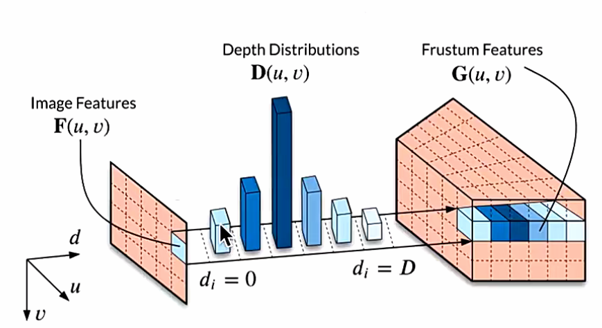
3. get_cam_feats得到(1, 6, 118, 32, 88, 80)。

• 输入：704*256的图片，以及depth
• 中间两个网络+深度概率分布（重要概念）
• 输出**（1，6，118，32，88，80）**

def get_cam_feats(self, x, d):B, N, C, fH, fW = x.shape  # x: (1, 6, 256, 32, 88), d: (1, 6, 1, 256, 704)# Reshaping and combining x and dd = d.view(B * N, C, *d.shape[2:])  # Shape: (6, 1, 256, 704)x = x.view(B * N, C, fH, fW)  # Shape: (6, 256, 32, 88)# Transformation of dd = self.dtransform(d)  # Transformation result (6, 64, 32, 88)# Concatenation of d and xx = torch.cat([d, x], dim=1)  # Shape: (6, 320, 32, 88)# Depth network operationx = self.depthnet(x)  # Depth processing result (6, 198, 32, 88)# Softmax normalization on depth datadepth = x[:, self.D].softmax(dim=1)  # Depth map (6, 118, 32, 88)# Combine depth and the input x for final outputx = depth.unsqueeze(1) * x[:, self.D : (self.D + self.C)].unsqueeze(2)  # Shape: (6, 118, 32, 88)# Adjust the final shape for returnx = x.view(B, N, self.D, fH, fW)  # Shape: (1, 6, 118, 32, 88)x = x.permute(1, 2, 3, 4, 0)  # Shape: (1, 6, 80, 118, 32, 88)return x

2.2.2 得到1, 6, 118, 32, 88, 3

1. 初始化中create_frustum采样

2. get_geometry采样点坐标(1, 6, 118, 32, 88, 3)转到lidar坐标系

   @force_fp32()def get_geometry(self,camera2lidar_rots,camera2lidar_trans,intrins,post_rots,post_trans,**kwargs,):B, N, _ = camera2lidar_trans.shape# undo post-transformation# B x N x D x H x W x 3points = self.frustum - post_trans.view(B, N, 1, 1, 1, 3)points = (torch.inverse(post_rots).view(B, N, 1, 1, 1, 3, 3).matmul(points.unsqueeze(-1)))# cam_to_lidarpoints = torch.cat((points[:, :, :, :, :, :2] * points[:, :, :, :, :, 2:3],points[:, :, :, :, :, 2:3],),5,)combine = camera2lidar_rots.matmul(torch.inverse(intrins))points = combine.view(B, N, 1, 1, 1, 3, 3).matmul(points).squeeze(-1)points += camera2lidar_trans.view(B, N, 1, 1, 1, 3)if "extra_rots" in kwargs:extra_rots = kwargs["extra_rots"]points = (extra_rots.view(B, 1, 1, 1, 1, 3, 3).repeat(1, N, 1, 1, 1, 1, 1).matmul(points.unsqueeze(-1)).squeeze(-1))if "extra_trans" in kwargs:extra_trans = kwargs["extra_trans"]points += extra_trans.view(B, 1, 1, 1, 1, 3).repeat(1, N, 1, 1, 1, 1)return points

4. bev_pool中一部分代码，把(1, 6, 118, 32, 88, 3)转到voxel坐标系

 @force_fp32()def bev_pool(self, geom_feats, x):B, N, D, H, W, C = x.shapeNprime = B * N  * D * H * W# flatten xx = x.reshape(Nprime, C)# flatten indicesgeom_feats = ((geom_feats - (self.bx - self.dx / 2.0)) / self.dx).long()geom_feats = geom_feats.view(Nprime, 3)batch_ix = torch.cat([torch.full([Nprime // B, 1], ix, device=x.device, dtype=torch.long)for ix in range(B)])geom_feats = torch.cat((geom_feats, batch_ix), 1)# filter out points that are outside boxkept = ((geom_feats[:, 0] >= 0)& (geom_feats[:, 0] < self.nx[0])& (geom_feats[:, 1] >= 0)& (geom_feats[:, 1] < self.nx[1])& (geom_feats[:, 2] >= 0)& (geom_feats[:, 2] < self.nx[2]))x = x[kept]geom_feats = geom_feats[kept]x = bev_pool(x, geom_feats, B, self.nx[2], self.nx[0], self.nx[1])# collapse Zfinal = torch.cat(x.unbind(dim=2), 1)return final

2.2.3 得到bev

划分360°*360°的格子，落到同格子的feature经过计算，变成bev

雷达处理流程总结

# bevfusion.py  →  BEVFusion.forward_singleif sensor == "camera":feature = self.extract_camera_features(img,points,camera2ego,lidar2ego,lidar2camera,lidar2image,camera_intrinsics,camera2lidar,img_aug_matrix,lidar_aug_matrix,metas,)
elif sensor == "lidar":feature = self.extract_lidar_features(points)
else:raise ValueError(f"unsupported sensor: {sensor}")

---

voxelize 函数的结果

输入

• x[0].shape = (207998, 5)
  说明：输入为 sample 与 sweep 增强后的点云。

输出

• feats.shape = (12683, 5)
  说明：由硬体素化得到的 (12683, 10, 5) 在长度为 10 的维度上取平均得到。对应 第 158 行；并在 第 161 行 做 contiguous（或等价处理）。

• coords.shape = (12683, 4)
  说明：维度顺序为 (batch_size, x, y, z)。与 batch_size 相关的调整见 第 149 行 与 第 131 行。

• sizes.shape = (12683,)
  说明：每个体素格内的点数量。

@torch.no_grad()
@force_fp32()
def voxelize(self, points):feats, coords, sizes = [], [], []for k, res in enumerate(points):ret = self.encoders["lidar"]["voxelize"](res)if len(ret) == 3:# hard voxelizec, f, n = retelse:assert len(ret) == 2f, c = retn = Nonefeats.append(f)coords.append(F.pad(c, (1, 0), mode="constant", value=k))if n is not None:sizes.append(n)feats = torch.cat(feats, dim=0)coords = torch.cat(coords, dim=0)if len(sizes) > 0:sizes = torch.cat(sizes, dim=0)if self.voxelize_reduce:feats = feats.sum(dim=1, keepdim=False) / sizes.type_as(feats).view(-1, 1)feats = feats.contiguous()return feats, coords, sizes

Lidar backbone

• 输入

  • 就是上面的输出

• 用输入

  • 构建成 SparsConvTensor，输入网络得到 BEV 特征

• 输出

  • spatial_features.shape：torch.Size([1, 256, 180, 180])

@auto_fp16(apply_to=("voxel_features",))def forward(self, voxel_features, coors, batch_size, **kwargs):"""Forward of SparseEncoder.Args:voxel_features (torch.float32): Voxel features in shape (N, C).coors (torch.int32): Coordinates in shape (N, 4),the columns in the order of (batch_idx, z_idx, y_idx, x_idx).batch_size (int): Batch size.Returns:dict: Backbone features."""coors = coors.int()input_sp_tensor = spconv.SparseConvTensor(voxel_features, coors, self.sparse_shape, batch_size)x = self.conv_input(input_sp_tensor)encode_features = []for encoder_layer in self.encoder_layers:x = encoder_layer(x)encode_features.append(x)# for detection head# [200, 176, 5] -> [200, 176, 2]out = self.conv_out(encode_features[-1])spatial_features = out.dense()N, C, H, W, D = spatial_features.shapespatial_features = spatial_features.permute(0, 1, 4, 2, 3).contiguous()spatial_features = spatial_features.view(N, C * D, H, W)return spatial_features

Sparse Conv

• 稀疏卷积github实现

  • 07spconv_explain.py 了解稀疏化（Lidar）

    • 了解 range 步长 1.0

    • 了解如何构建 boardmix 样的 SparsTensor

  • 07spconv_2d.py 了解如何直接构建 SparsConvTensor，构建网络

subm模式

使用说明

简要API说明

import spconv.pytorch as spconv
from spconv.pytorch import functional as Fsp
from torch import nn
from spconv.pytorch.utils import PointToVoxel
from spconv.pytorch.hash import HashTable

层 API	常见用途	稠密版	备注
spconv.SparseConv3d	下采样	nn.Conv3d	使用 indice_key 保存数据以便反向使用
spconv.SubMConv3d	卷积	N/A	使用 indice_key 保存数据以便重用
spconv.SparseInverseConv3d	上采样	N/A	使用预先保存的 indice_key 进行上采样
spconv.SparseConvTranspose3d	上采样（生成模型）	nn.ConvTranspose3d	非常慢且无法恢复原始点云
spconv.SparseMaxPool3d	下采样	nn.MaxPool3d	使用 indice_key 保存数据以便反向使用
spconv.SparseSequential	容器	nn.Sequential	支持上面的层和 nn.ReLU, nn.BatchNorm, ...
spconv.SparseGlobalMaxPool	全局池化	N/A	返回稠密张量而非 SparseConvTensor
spconv.SparseGlobalAvgPool	全局池化	N/A	返回稠密张量而非 SparseConvTensor

功能 API	用法
Fsp.sparse_add	对具有相同形状但不同索引的稀疏张量进行加法运算

输入 API	用法
PointToVoxel	点云转为体素

杂项 API	用法
HashTable	哈希表，一个槽位

层 API	torchsparse	MinkowskiEngine
spconv.SparseConv3d	Conv3d(stride!=1, transpose=False)	MinkowskiConvolution(stride!=1)
spconv.SubMConv3d	Conv3d(stride=1, transpose=False)	MinkowskiConvolution(stride=1)
spconv.SparseInverseConv3d	Conv3d(stride!=1, transpose=True)	MinkowskiConvolutionTranspose
spconv.SparseConvTranspose3d	N/A	MinkowskiConvolutionTranspose
spconv.SparseMaxPool3d	N/A	MinkowskiMaxPooling

概念

• 稀疏卷积张量：类似于混合型 torch.sparse_coo_tensor，但有两点区别：1. 稀疏卷积张量只有一个稠密维度，2. 稀疏卷积张量的索引是转置的，详细请参见 PyTorch 文档。

• 稀疏卷积：相当于将稀疏卷积张量转换为稠密时执行稠密卷积。稀疏卷积仅在有效数据上运行计算。

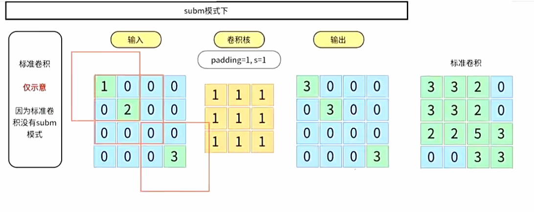
• 子流形卷积（SubMConv）：类似于稀疏卷积，但保持索引不变。可以想象你将相同的空间结构复制到输出，然后迭代它们，通过卷积规则获取输入坐标，最后仅在这些输出坐标上应用卷积。

SparseConvTensor

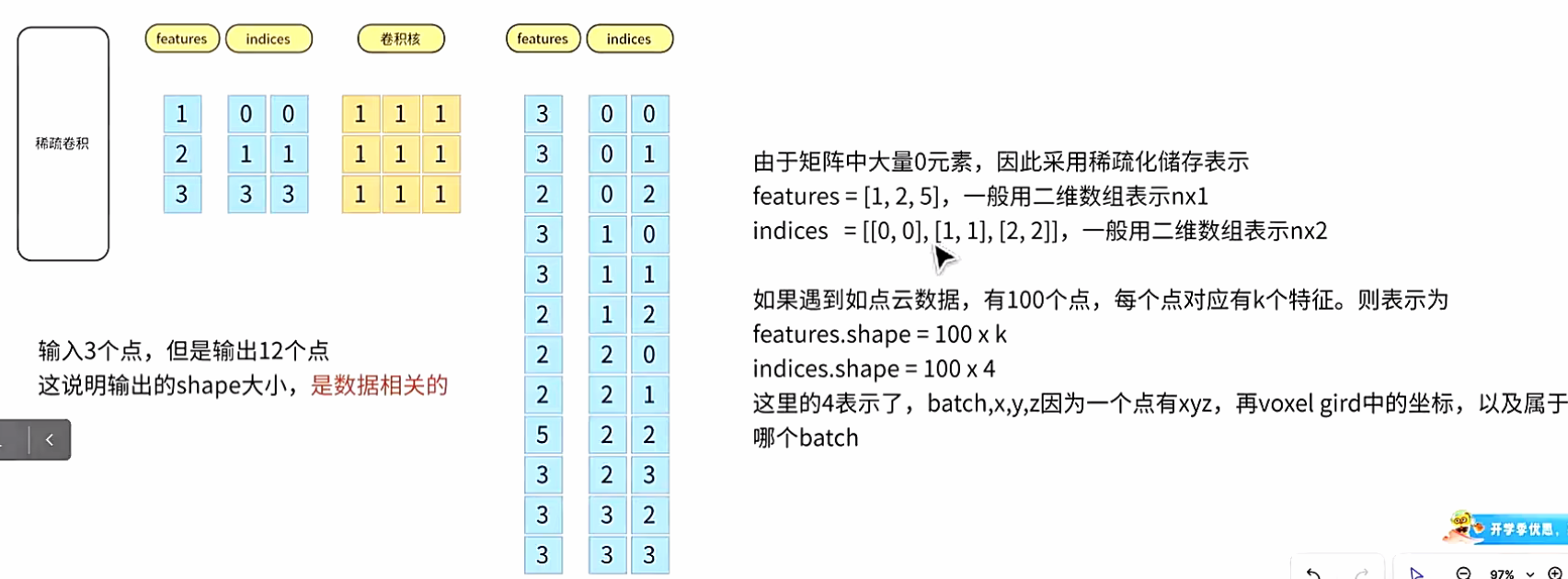
• features：形状为 [N, num_channels] 的张量。

• indices：形状为 [N, (batch_idx + x + y + z)] 的坐标张量，包含批次轴。请注意，坐标的 xyz 顺序必须与空间形状和卷积参数（如卷积核大小）匹配。

import spconv.pytorch as spconv
features = # 你的特征，形状为 [N, num_channels]
indices = # 你的索引/坐标，形状为 [N, ndim + 1]，批次索引必须放在 indices[:, 0] 中
spatial_shape = # 稀疏张量的空间形状，spatial_shape[i] 为 indices[:, 1 + i] 的形状。
batch_size = # 稀疏张量的批次大小。
x = spconv.SparseConvTensor(features, indices, spatial_shape, batch_size)
x_dense_NCHW = x.dense() # 将稀疏张量转换为稠密 NCHW 张量。

稀疏卷积

import spconv.pytorch as spconv
from torch import nn
class ExampleNet(nn.Module):def __init__(self, shape):super().__init__()self.net = spconv.SparseSequential(spconv.SparseConv3d(32, 64, 3), # 类似于 nn.Conv3d，但不支持 groupnn.BatchNorm1d(64), # 非空间层可以直接用于 SparseSequential。nn.ReLU(),spconv.SubMConv3d(64, 64, 3, indice_key="subm0"),nn.BatchNorm1d(64),nn.ReLU(),# 使用子流形卷积时，它们的索引可以共享，以节省生成索引的时间。spconv.SubMConv3d(64, 64, 3, indice_key="subm0"),nn.BatchNorm1d(64),nn.ReLU(),spconv.SparseConvTranspose3d(64, 64, 3, 2),nn.BatchNorm1d(64),nn.ReLU(),spconv.ToDense(), # 将稀疏张量转换为稠密张量并转换为 NCHW 格式。nn.Conv3d(64, 64, 3),nn.BatchNorm1d(64),nn.ReLU(),)self.shape = shapedef forward(self, features, coors, batch_size):coors = coors.int() # 与 torch 不同，该库只接受整数坐标。x = spconv.SparseConvTensor(features, coors, self.shape, batch_size)return self.net(x)# .dense()

逆卷积

逆稀疏卷积是指稀疏卷积的反向操作。逆卷积的输出包含与稀疏卷积输入相同的索引。

警告 SparseInverseConv 不等于 SparseConvTranspose。SparseConvTranspose 相当于 PyTorch 中的 ConvTranspose，但 SparseInverseConv 不一样。

逆卷积通常用于语义分割。

class ExampleNet(nn.Module):def __init__(self, shape):super().__init__()self.net = spconv.SparseSequential(spconv.SparseConv3d(32, 64, 3, 2, indice_key="cp0"),spconv.SparseInverseConv3d(64, 32, 3, indice_key="cp0"), # 需要提供卷积核大小来创建权重)self.shape = shapedef forward(self, features, coors, batch_size):coors = coors.int()x = spconv.SparseConvTensor(features, coors, self.shape, batch_size)return self.net(x)

生成模型用法

SparseConvTranspose（标准上采样）应仅在生成模型中使用。你需要使用分类器来检查输出坐标是否为空，然后将该稀疏张量的批次索引（或 xyz）设置为负值。

1. 使用 SparseConvTranspose 上采样你的稀疏卷积张量，这将生成大量的点。

2. 使用分类器获取有效的索引。

3. 使用 select_by_index 生成新的稀疏卷积张量。

常见错误

• 问题 #467

class WrongNet(nn.Module):def __init__(self, shape):super().__init__()self.Encoder = spconv.SparseConv3d(channels, channels, kernel_size=3, stride=2, indice_key="cp1",algo=algo)self.Sparse_Conv = spconv.SparseConv3d(channels, channels, kernel_size=3, stride=1,algo=algo)self.Decoder = spconv.SparseInverseConv3d(channels, channels, kernel_size=3, indice_key="cp1",algo=algo)   def forward(self, sparse_tensor):encoded = self.Encoder(sparse_tensor)s_conv = self.Sparse_Conv(encoded)return self.Decoder(s_conv).featuresclass CorrectNet(nn.Module):def __init__(self, shape):super().__init__()self.Encoder = spconv.SparseConv3d(channels, channels, kernel_size=3, stride=2, indice_key="cp1",algo=algo)self.Sparse_Conv = spconv.SparseConv3d(channels, channels, kernel_size=3, stride=1, indice_key="cp2",algo=algo)self.Sparse_Conv_Decoder = spconv.SparseInverseConv3d(channels, channels, kernel_size=3, indice_key="cp2",algo=algo)   self.Decoder = spconv.SparseInverseConv3d(channels, channels, kernel_size=3, indice_key="cp1",algo=algo)   def forward(self, sparse_tensor):encoded = self.Encoder(sparse_tensor)s_conv = self.Sparse_Conv(encoded)return self.Decoder(self.Sparse_Conv_Decoder(s_conv)).features

在 ExampleNet 中的 Sparse_Conv 改变了 Encoder 输出的空间结构，因此我们无法通过 Decoder 反向得到 Encoder 的输入，我们需要通过 Sparse_Conv.output 反向到 Encoder.output，然后再通过 Decoder 反向到 Encoder.input。

稀疏加法

在语义分割网络中，我们可能会使用 conv1x3、3x1 和 3x3 在一个块中，但由于常规加法需要相同的索引，因此无法将这些层的结果加在一起。

spconv >= 2.1.17 提供了一种操作，可以对具有不同索引的稀疏张量进行加法（形状必须相同），但有一些限制：

from spconv.pytorch import functional as Fsp
res_1x3 = conv1x3(x)
res_3x1 = conv3x1(x)
# 错误
# 因为我们无法“反向”这个操作
wrong_usage_cant_inverse = Fsp.sparse_add(res_1x3, res_3x1)# 正确
# res_3x3 已经包含了 res_1x3 和 res_3x1 的所有索引，
# 所以输出的空间结构不会改变，我们可以“反向”回去。
res_3x3 = conv3x3(x)
correct = Fsp.sparse_add(res_1x3, res_3x1, res_3x3)

如果你使用的网络没有 SparseInverseConv，上面的限制不存在，sparse_add 的唯一缺点是它比简单的对齐加法慢。

快速混合精度训练

见 example/mnist_sparse。我们支持 torch.cuda.amp。

工具函数

• 点云转换为体素

spconv 中的体素生成器生成 ZYX 顺序的索引，参数格式为 XYZ。

生成的索引不包括批次轴，你需要自己添加。

请参见 examples/voxel_gen.py 了解更多示例。

from spconv.pytorch.utils import PointToVoxel, gather_features_by_pc_voxel_id
# 这个生成器生成 ZYX 顺序的索引。
gen = PointToVoxel(vsize_xyz=[0.1, 0.1, 0.1], coors_range_xyz=[-80, -80, -2, 80, 80, 6], num_point_features=3, max_num_voxels=5000, max_num_points_per_voxel=5)
pc = np.random.uniform(-10, 10, size=[1000, 3])
pc_th = torch.from_numpy(pc)
voxels, coords, num_points_per_voxel = gen(pc_th, empty_mean=True)

如果你想为点云的每个点获取标签，你需要使用另一个函数获取 pc_voxel_id 并根据语义分割结果收集特征：

voxels, coords, num_points_per_voxel, pc_voxel_id = gen.generate_voxel_with_id(pc_th, empty_mean=True)
seg_features = YourSegNet(...)
# 如果体素 id 无效（点不在范围内，或体素中没有空间）
# 特征将为零。
point_features = gather_features_by_pc_voxel_id(seg_features, pc_voxel_id)

是一个使用 SparseConvTensor 的简单案例：

安装 spconv

首先，确保你已安装 spconv 库，如果没有安装，可以通过以下命令进行安装：

pip install spconv

代码示例

这个示例展示了如何使用 SparseConvTensor 创建一个稀疏卷积网络。

import torch
import spconv.pytorch as spconv
from torch import nn# 定义一个简单的稀疏卷积网络
class SparseConvNet(nn.Module):def __init__(self, spatial_shape):super().__init__()# 使用稀疏卷积序列self.net = spconv.SparseSequential(# 稀疏卷积层spconv.SparseConv3d(32, 64, 3),  # 输入通道32，输出通道64，卷积核大小为3nn.ReLU(),  # 非稀疏的激活层spconv.SubMConv3d(64, 64, 3, indice_key="subm0"),  # 子流形卷积nn.ReLU(),spconv.SparseConv3d(64, 128, 3),  # 再次使用稀疏卷积层nn.ReLU(),spconv.ToDense(),  # 转换为稠密张量nn.Conv3d(128, 128, 3),  # 普通的稠密卷积nn.ReLU())self.spatial_shape = spatial_shapedef forward(self, features, coors, batch_size):# 将输入的点云特征和坐标转化为 SparseConvTensorcoors = coors.int()  # 坐标必须是整数sparse_tensor = spconv.SparseConvTensor(features, coors, self.spatial_shape, batch_size)# 通过网络进行前向传播return self.net(sparse_tensor)# 假设我们有以下输入数据
batch_size = 1
features = torch.rand((10, 32))  # 10个点，每个点有32个特征
coors = torch.tensor([[0, 1, 2, 3], [0, 2, 3, 4], [0, 3, 4, 5], [0, 4, 5, 6], [0, 5, 6, 7],[0, 6, 7, 8], [0, 7, 8, 9], [0, 8, 9, 10], [0, 9, 10, 11], [0, 10, 11, 12]])  # 假设的点云坐标
spatial_shape = [16, 16, 16]  # 假设的空间形状，3D体素网格大小
model = SparseConvNet(spatial_shape)# 执行前向传播
output = model(features, coors, batch_size)
print(output.shape)  # 输出结果的形状

解释

1. SparseConvTensor 创建：

   • features 是一个二维张量，包含每个点的特征。假设有 10 个点，每个点有 32 个特征。

   • coors 是一个包含坐标的张量，每个点有 4 个坐标值（包括批次索引）。

   • spatial_shape 定义了稀疏张量的空间形状，在此示例中为 16x16x16。

2. 稀疏卷积层：

   • 使用 spconv.SparseConv3d 和 spconv.SubMConv3d 进行稀疏卷积。

   • spconv.SparseConv3d(32, 64, 3) 表示输入通道为 32，输出通道为 64，卷积核大小为 3。

   • spconv.ToDense() 将稀疏张量转换为稠密张量，以便进行后续的稠密卷积处理。

3. 前向传播：

   • 使用 spconv.SparseConvTensor(features, coors, self.spatial_shape, batch_size) 将点云特征和坐标转换为稀疏卷积张量（SparseConvTensor）。

   • 通过定义的网络结构进行前向传播。

输出

torch.Size([1, 128, 8, 8, 8])  # 输出的形状（稠密张量的形状）

此代码创建了一个简单的稀疏卷积网络并对一个小的点云数据进行前向传播。

1. features（特征）

features 是一个包含每个点的特征的张量，它的形状为 [N, num_channels]，其中：

• N 是点的数量（每个点都有一个特征向量）。

• num_channels 是每个点的特征维度，通常是每个点的属性值（如颜色、强度等）。

示例：假设我们有 5 个点，每个点有 3 个特征，features 的形状就是 [5, 3]。

features = torch.tensor([[0.1, 0.2, 0.3],  # 点 1[0.4, 0.5, 0.6],  # 点 2[0.7, 0.8, 0.9],  # 点 3[1.0, 1.1, 1.2],  # 点 4[1.3, 1.4, 1.5]   # 点 5
], dtype=torch.float32)

这里，我们有 5 个点，每个点有 3 个特征（num_channels=3）。

2. indices（索引）

indices 是一个包含每个点坐标的张量，形状为 [N, ndim + 1]，其中：

• N 是点的数量（和 features 中的点数量一致）。

• ndim 是坐标的维度，这里是 3D 坐标，所以 ndim=3（即每个点有 3 个坐标值：x, y, z）。

• +1 是为了包含批次索引（batch index）。indices 的第一列存储批次索引，后面每一列存储点的 x, y, z 坐标。

示例：假设我们有 5 个点，并且这些点的坐标分别为（x, y, z）。批次索引是 0（假设所有点属于同一个批次）。

indices = torch.tensor([[0, 1, 2, 3],  # 点 1，坐标 (x=1, y=2, z=3)[0, 4, 5, 6],  # 点 2，坐标 (x=4, y=5, z=6)[0, 7, 8, 9],  # 点 3，坐标 (x=7, y=8, z=9)[0, 10, 11, 12],# 点 4，坐标 (x=10, y=11, z=12)[0, 13, 14, 15] # 点 5，坐标 (x=13, y=14, z=15)
], dtype=torch.int32)

在 indices 中：

• 第一列是批次索引（所有点属于批次 0）。

• 后三列分别是点的 x, y, z 坐标。

3. spatial_shape（空间形状）

spatial_shape 是一个列表或元组，表示稀疏张量的空间大小。在此示例中，我们使用 3D 空间，所以 spatial_shape 是一个包含 3 个数字的列表，表示 x, y, z 轴的大小。

示例：假设我们有一个 16x16x16 的体素网格，每个坐标轴的大小为 16。

spatial_shape = [16, 16, 16]

spatial_shape 定义了稀疏张量中每个维度的最大尺寸，这意味着 indices 中的坐标值应该小于或等于该维度的大小。

4. batch_size（批次大小）

batch_size 是指稀疏张量中的批次数量。在 3D 点云处理任务中，通常一个批次包含多个点云样本。如果只处理一个点云，则 batch_size 为 1。

示例：假设我们有一个批次，其中只有一个点云，则 batch_size=1。

batch_size = 1

综合示例

现在，我们将所有这些部分综合到一起，创建一个 SparseConvTensor：

import torch
import spconv.pytorch as spconv# 假设的输入数据
features = torch.tensor([[0.1, 0.2, 0.3],  # 点 1[0.4, 0.5, 0.6],  # 点 2[0.7, 0.8, 0.9],  # 点 3[1.0, 1.1, 1.2],  # 点 4[1.3, 1.4, 1.5]   # 点 5
], dtype=torch.float32)indices = torch.tensor([[0, 1, 2, 3],  # 点 1，坐标 (x=1, y=2, z=3)[0, 4, 5, 6],  # 点 2，坐标 (x=4, y=5, z=6)[0, 7, 8, 9],  # 点 3，坐标 (x=7, y=8, z=9)[0, 10, 11, 12],# 点 4，坐标 (x=10, y=11, z=12)[0, 13, 14, 15] # 点 5，坐标 (x=13, y=14, z=15)
], dtype=torch.int32)spatial_shape = [16, 16, 16]  # 体素网格大小
batch_size = 1  # 只有一个批次# 创建 SparseConvTensor
sparse_tensor = spconv.SparseConvTensor(features, indices, spatial_shape, batch_size)# 打印稀疏张量的特性
print(f"SparseConvTensor Features: {sparse_tensor.features.shape}")
print(f"SparseConvTensor Indices: {sparse_tensor.indices.shape}")
print(f"SparseConvTensor Spatial Shape: {sparse_tensor.spatial_shape}")

解释：

1. features：包含了每个点的特征，共有 5 个点，每个点有 3 个特征。

2. indices：包含了每个点的坐标，共有 5 个点，每个点有 4 个值（批次索引和 3D 坐标）。

3. spatial_shape：定义了稀疏张量的空间大小，这里是 16x16x16，意味着每个坐标值（x, y, z）都应该在 [0, 16) 之间。

4. batch_size：只有一个批次。

输出：

SparseConvTensor Features: torch.Size([5, 3])
SparseConvTensor Indices: torch.Size([5, 4])
SparseConvTensor Spatial Shape: [16, 16, 16]

这里，SparseConvTensor 中包含了特征、索引和空间形状。features 和 indices 以稀疏方式存储，以便进行稀疏卷积操作。