Python11-集成学习

提示：文章写完后，目录可以自动生成，如何生成可参考右边的帮助文档

---

前言

1. 介绍

集成学习通过建⽴⼏个模型来解决单⼀预测问题。它的⼯作原理是⽣成多个分类器/模型，各⾃独⽴地学习和作出预
测。这些预测最后结合成组合预测，因此优于任何⼀个单分类的做出预测

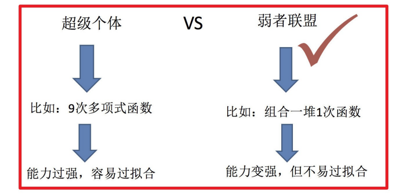
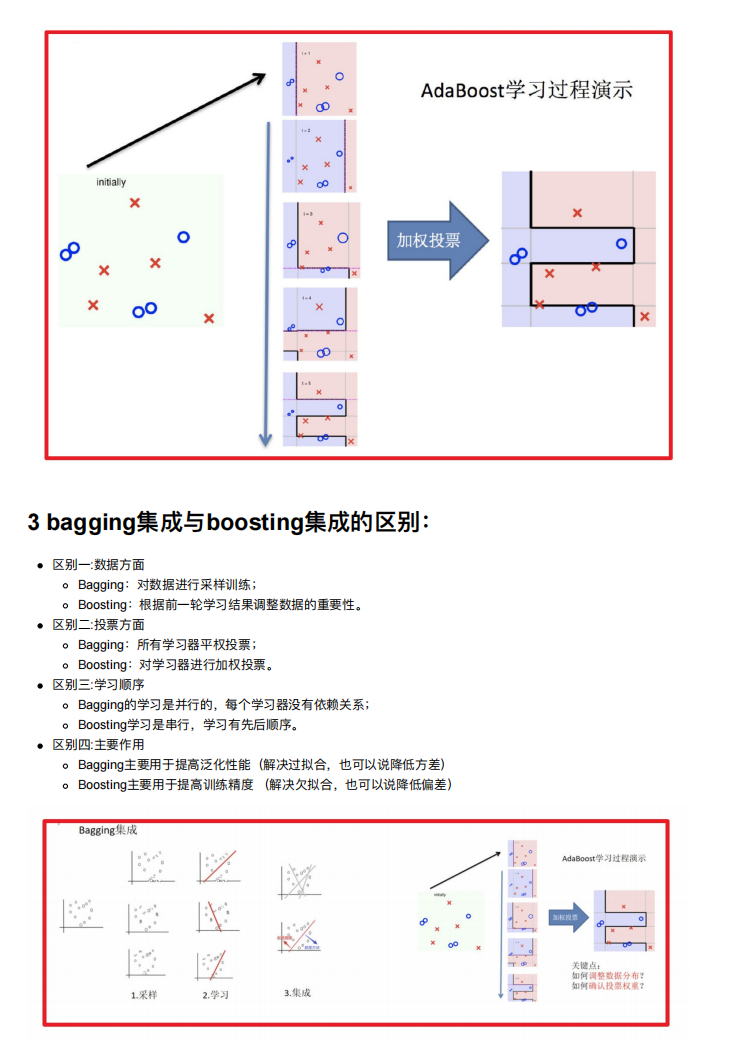
1.1 集成学习中boosting和Bagging

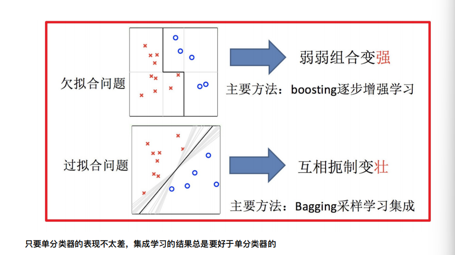
只要单分类器的表现不太差，集成学习的结果总是要好于单分类器的

2. Bagging和随机森林

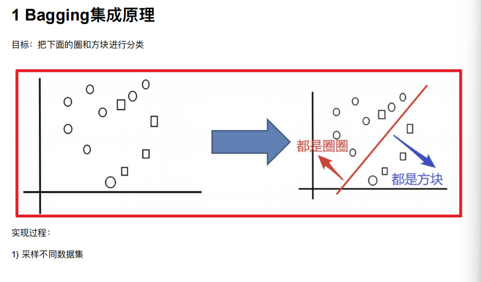
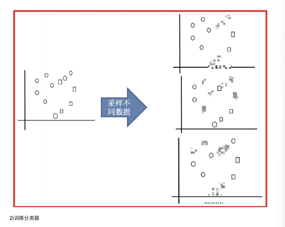
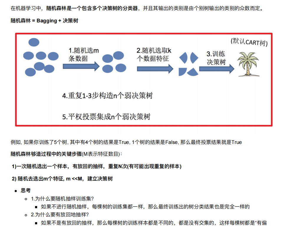
2.1 随机森林构造过程

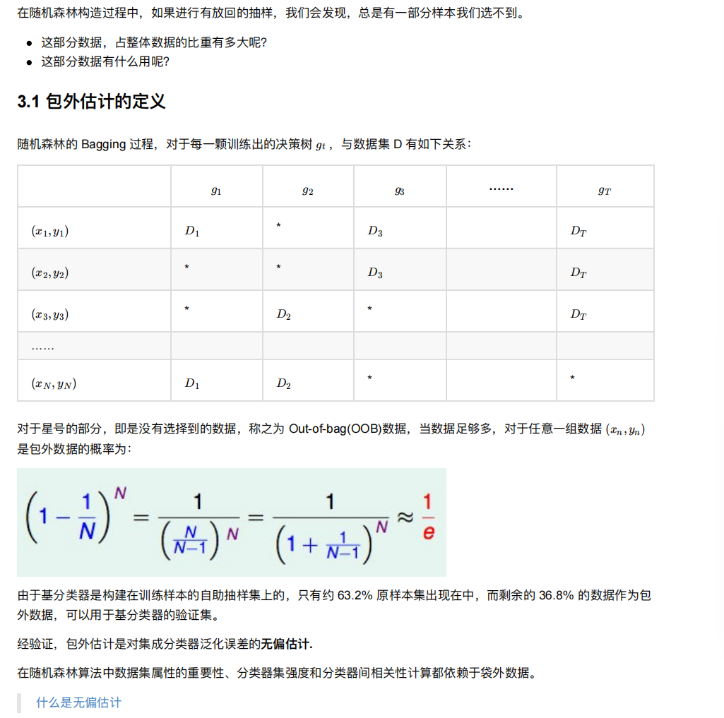
2.2 包外估计

2.3 随机森林api介绍

sklearn.ensemble.RandomForestClassifier(n_estimators=10, criterion=’gini’, max_depth=None, bootstrap=True,random_state=None, min_samples_split=2)

n_estimators：表示是多少棵决策树集成森林

Criterion：string，可选(default =“gini”)
分割特征的测量⽅法

max_depth：integer或None，可选(默认=⽆)
树的最⼤深度 5,8,15,25,30

max_features="auto”,每个决策树的最⼤特征数量

If "auto", then max_features=sqrt(n_features) .
If "sqrt", then max_features=sqrt(n_features) (same as "auto").
If "log2", then max_features=log2(n_features) .
If None, then max_features=n_features .

bootstrap：boolean，optional(default = True)
是否在构建树时使⽤放回抽样

min_samples_split 内部节点再划分所需最⼩样本数
这个值限制了⼦树继续划分的条件，如果某节点的样本数少于min_samples_split，则不会继续再尝试选择最优特征来进⾏划分，默认是2。
如果样本量不⼤，不需要管这个值。如果样本量数量级⾮常⼤，则推荐增⼤这个值。

min_samples_leaf 叶⼦节点的最⼩样本数
这个值限制了叶⼦节点最少的样本数，如果某叶⼦节点数⽬⼩于样本数，则会和兄弟节点⼀起被剪枝，默认是1。
叶是决策树的末端节点。 较⼩的叶⼦使模型更容易捕捉训练数据中的噪声。

min_impurity_split: 节点划分最⼩不纯度
这个值限制了决策树的增⻓，如果某节点的不纯度(基于基尼系数，均⽅差)⼩于这个阈值，则该节点不再⽣成⼦节点。即为叶⼦节点

上⾯决策树参数中最重要的包括
最⼤特征数max_features，
最⼤深度max_depth，
内部节点再划分所需最⼩样本数min_samples_split
叶⼦节点最少样本数min_samples_leaf。

2.4 随机森林预测案例

还是选择的原来的泰坦尼克号数据

#实例化一个随机森林
from sklearn.ensemble import RandomForestClassifier
rf = RandomForestClassifier()

#通过超参数调优
from sklearn.model_selection import GridSearchCV
param = {"n_estimators":[100,120,300],"max_depth":[3,7,10]}
gc = GridSearchCV(rf,param_grid=param,cv=3)
gc.fit(x_train,y_train)

n_estimators：控制随机森林中决策树的数量（这里尝试 100、120、300 三档）。树越多通常性能越好，但计算成本也越高

max_depth：控制每棵决策树的最大深度（这里尝试 3、7、10 三档）。深度越小，模型越简单（不易过拟合）；深度越大，模型越复杂（可能过拟合）
param_grid=param, # 要搜索的超参数组合
网格搜索（GridSearchCV）
交叉验证（cv=3）

这个意思就是利用网格搜索找出最好的随机森林（从三个中找出来）gc

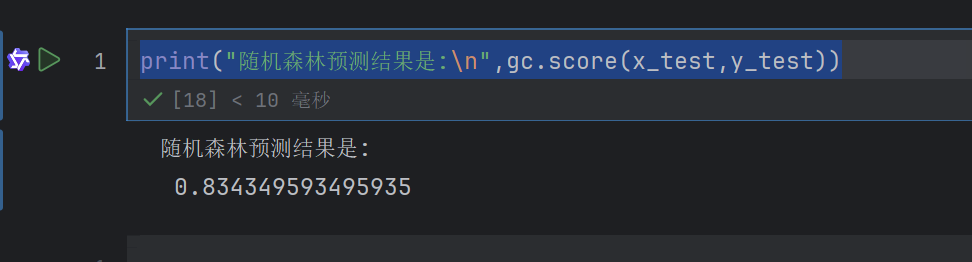
print("随机森林预测结果是:\n",gc.score(x_test,y_test))

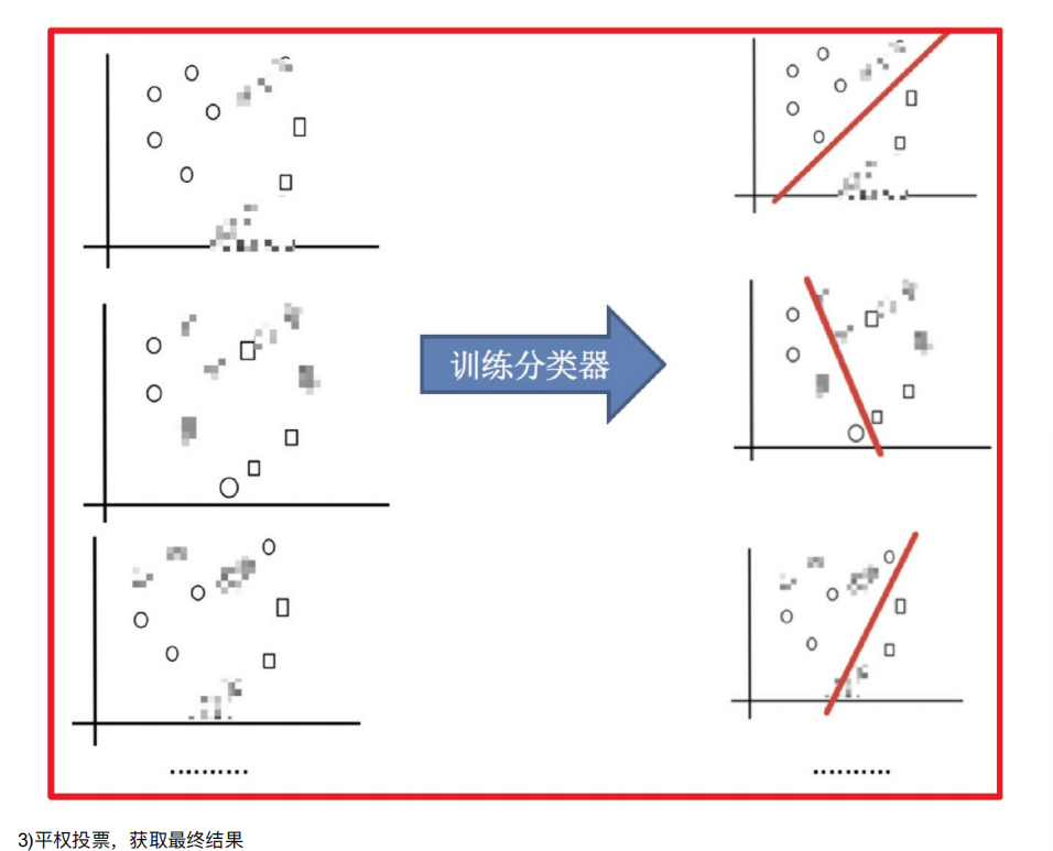
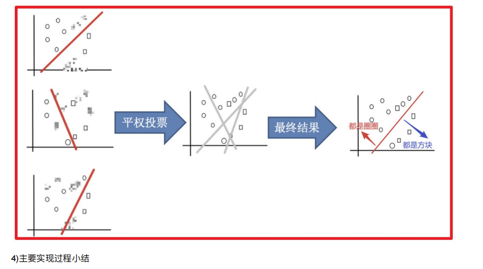
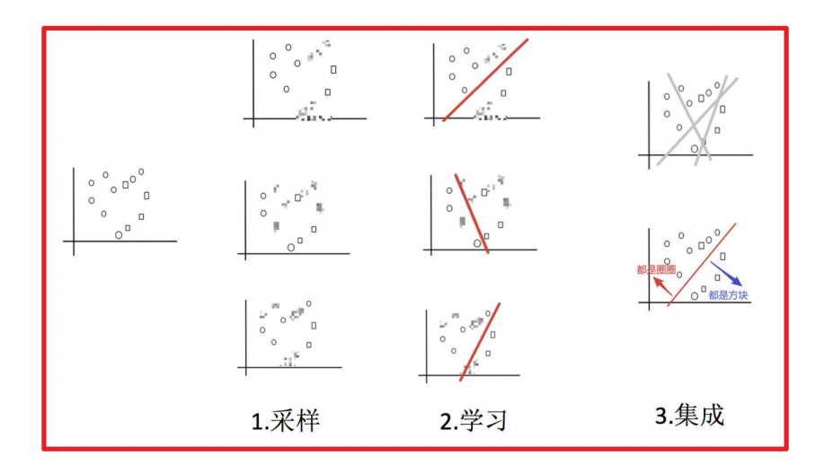
Bagging + 决策树/线性回归/逻辑回归/深度学习… = bagging集成学习⽅法
经过上⾯⽅式组成的集成学习⽅法:

1. 均可在原有算法上提⾼约2%左右的泛化正确率
2. 简单, ⽅便, 通⽤

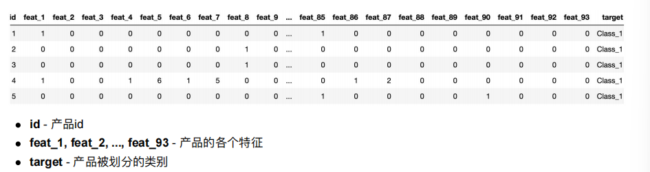
3. otto案例介绍

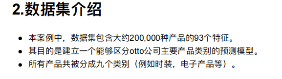
4.1 流程分析

获取数据
数据基本处理
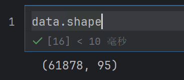
数据量⽐较⼤，尝试是否可以进⾏数据分割
转换⽬标值表示⽅式
模型训练
模型基本训练

import numpy as np
import pandas as pd
import matplotlib.pyplot as plt

#图像可视化，查看数据分布
import seaborn as sns
sns.countplot(x=data.target)
plt.show()

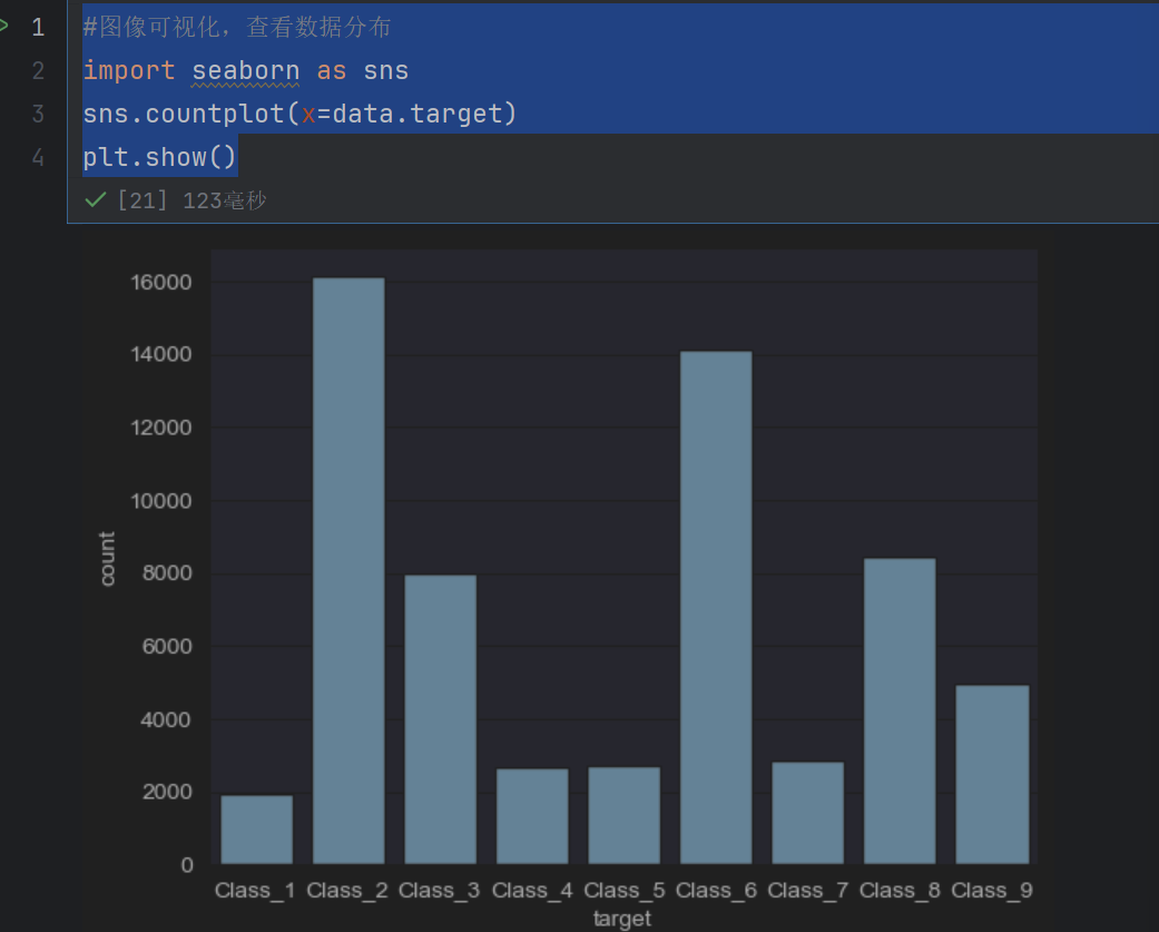
我们发现数据不平衡，类别不均衡–》纵坐标为数量

4.2 数据基本处理

#数据基本处理，数据已经脱敏，不在需要特殊处理
#数据截取
new1_data = data[:10000]
new1_data

这样直接截取前面10000是肯定不可以的

#数据基本处理，数据已经脱敏，不在需要特殊处理
#数据截取:随机欠采样
y = data["target"]
x=data.drop(["id","target"],axis=1)

y就是目标值了
x就少了两列了

#欠采样获取数据
from imblearn.under_sampling import  RandomUnderSampler
rus = RandomUnderSampler(random_state=42)
x_res, y_res = rus.fit_resample(x, y)

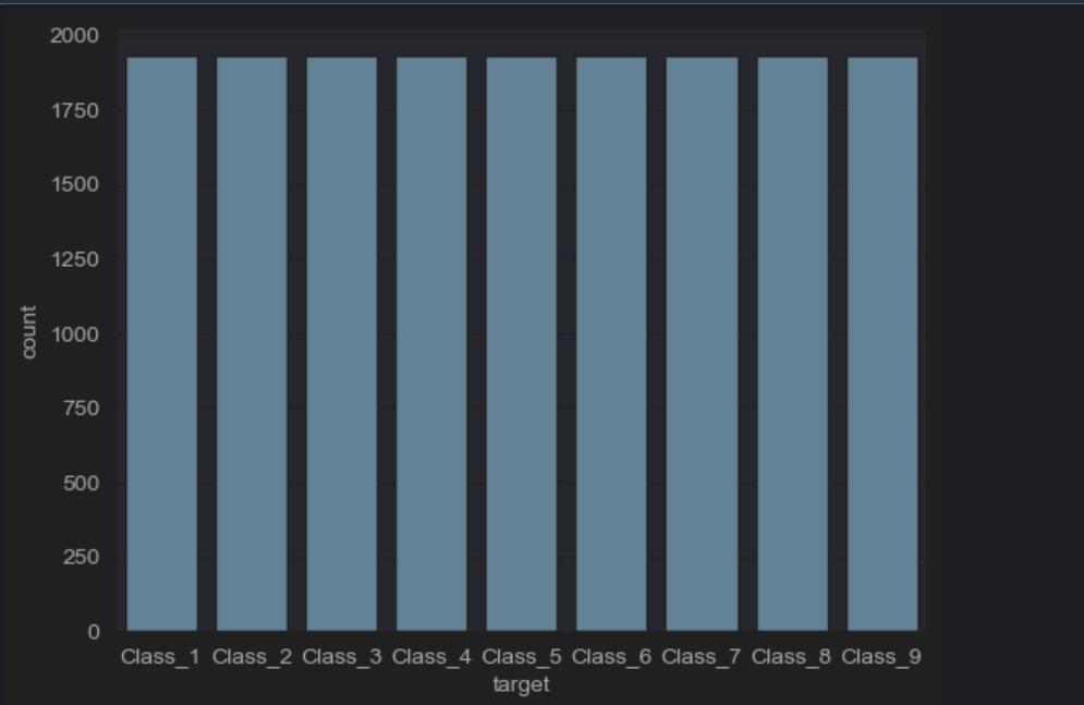
#图像可视化，查看数据分布
import seaborn as sns
sns.countplot(x=y_res)
plt.show()

欠采样是通过减少多数类样本数量，使不同类别样本数量趋于平衡的方法

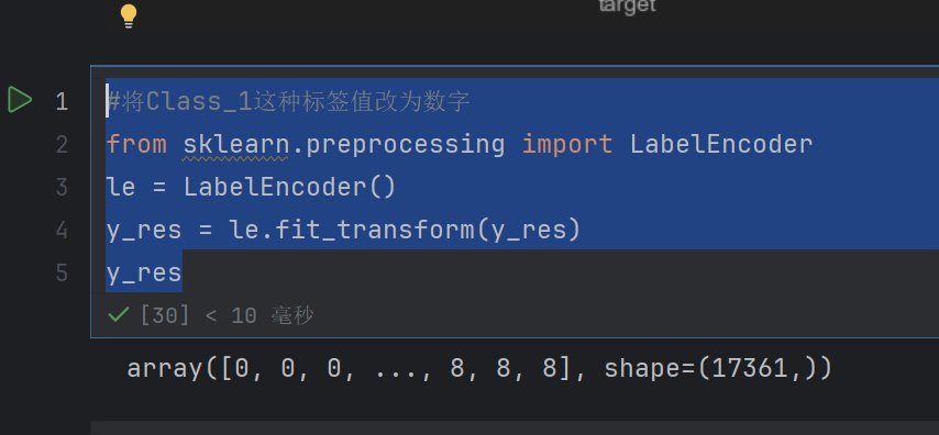
#将Class_1这种标签值改为数字
from sklearn.preprocessing import LabelEncoder
le = LabelEncoder()
y_res = le.fit_transform(y_res)
y_res

拟合（fit）：
分析输入的标签数据（y_res），提取其中所有唯一的类别（比如 Class_1、Class_2、Class_3 等）。
为每个唯一类别分配一个对应的整数（通常从 0 开始依次编号），建立 “类别→数字” 的映射关系。例如：
Class_1 → 0
Class_2 → 1
Class_3 → 2
转换（transform）：
根据第一步建立的映射关系，将原始标签数据（如 Class_1、Class_2 等）转换为对应的数字。
最终输出全是数字的标签数组（y_res），方便机器学习模型处理（大多数模型只能接受数值型输入）

#分割数据，测试集和训练集
from sklearn.model_selection import train_test_split
x_train, x_test, y_train, y_test = train_test_split(x_res, y_res, test_size=0.2, random_state=42)

4.3 模型基本训练

#模型基本训练
from sklearn.ensemble import  RandomForestClassifier
rf=RandomForestClassifier(oob_score= True)
rf.fit(x_train,y_train)

oob_score=True 是一个非常实用的参数，其中 OOB 是 Out-of-Bag（袋外样本）
随机森林在构建每棵决策树时，会通过 Bootstrap 抽样（有放回的随机抽样）从训练集中抽取部分样本作为该树的训练数据。
那些未被抽到的样本，就称为这棵树的 “袋外样本”（OOB 样本）。
由于是随机抽样，每棵树都会有自己的 OOB 样本，整体上约有 37% 的样本会成为某棵树的 OOB 样本（数学上的近似结果）。
当设置 oob_score=True 时，模型会在训练完成后：
用每棵树的 OOB 样本作为 “验证集”，对该树进行预测；
综合所有树的预测结果（对 OOB 样本的预测），计算出一个整体的模型性能得分（默认是准确率，分类问题）。
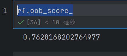
这个得分被称为 OOB 分数，可以通过 rf.oob_score_ 查看

rf.oob_score_

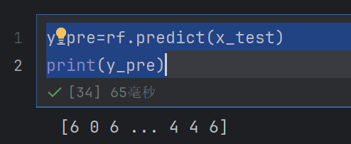
y_pre=rf.predict(x_test)
print(y_pre)

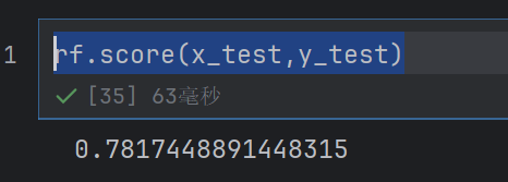
rf.score(x_test,y_test)

#图像可视化，查看数据分布
import seaborn as sns
sns.countplot(x=y_pre)
plt.show()

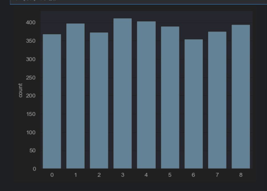
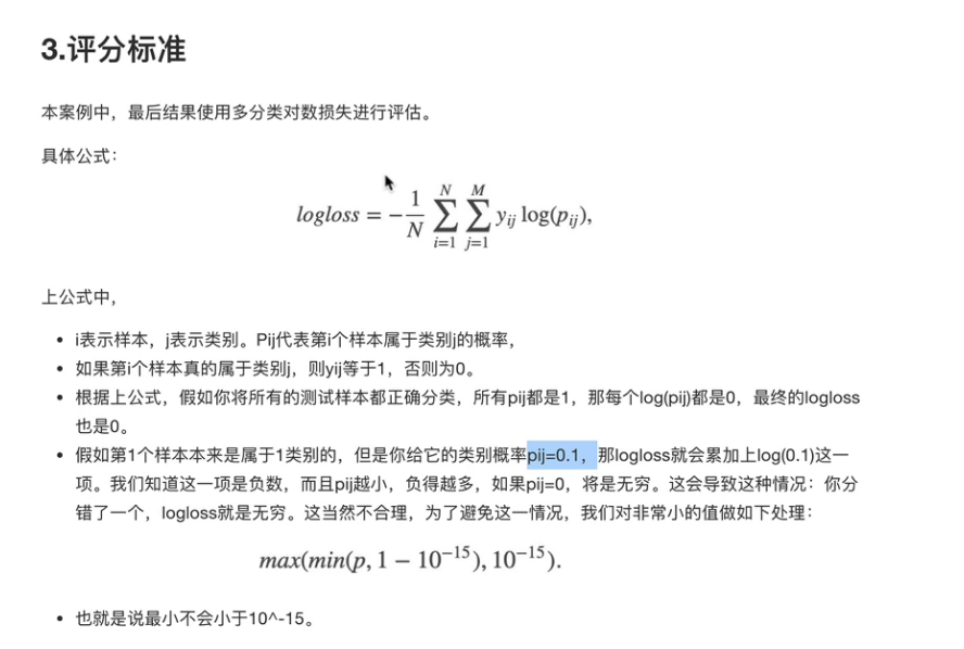
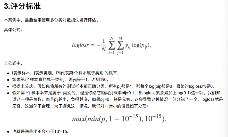
但是我们要用这个logloss进行评估才可以

#logloss模型评估
from sklearn.metrics import log_loss
log_loss(y_test,y_pre,epsilon=1e-15,normalize=True)

epsilon=1e-15：用于数值稳定性的极小值。因为对数损失计算中包含 log§ 操作，当 p 接近 0 时，log§ 会趋于无穷大。这个参数会将预测概率限制在 [epsilon, 1-epsilon] 范围内，避免计算错误。
normalize=True：是否对损失值进行归一化。
若为 True（默认），返回的是平均对数损失（总损失除以样本数量）。
若为 False，返回的是总对数损失（所有样本的损失之和）。

但是注意第二个参数必须是oneHot编码的显示的

所以这样是不行的

from sklearn.preprocessing import  OneHotEncoder
onehot = OneHotEncoder(sparse_output= False)
y_test1=onehot.fit_transform(y_test.reshape(-1,1))
y_pre1=onehot.transform(y_pre.reshape(-1,1))

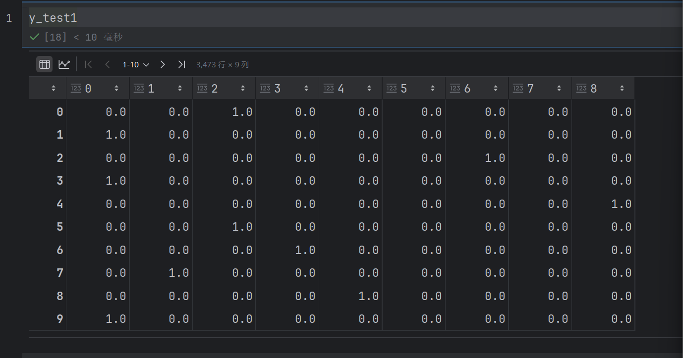
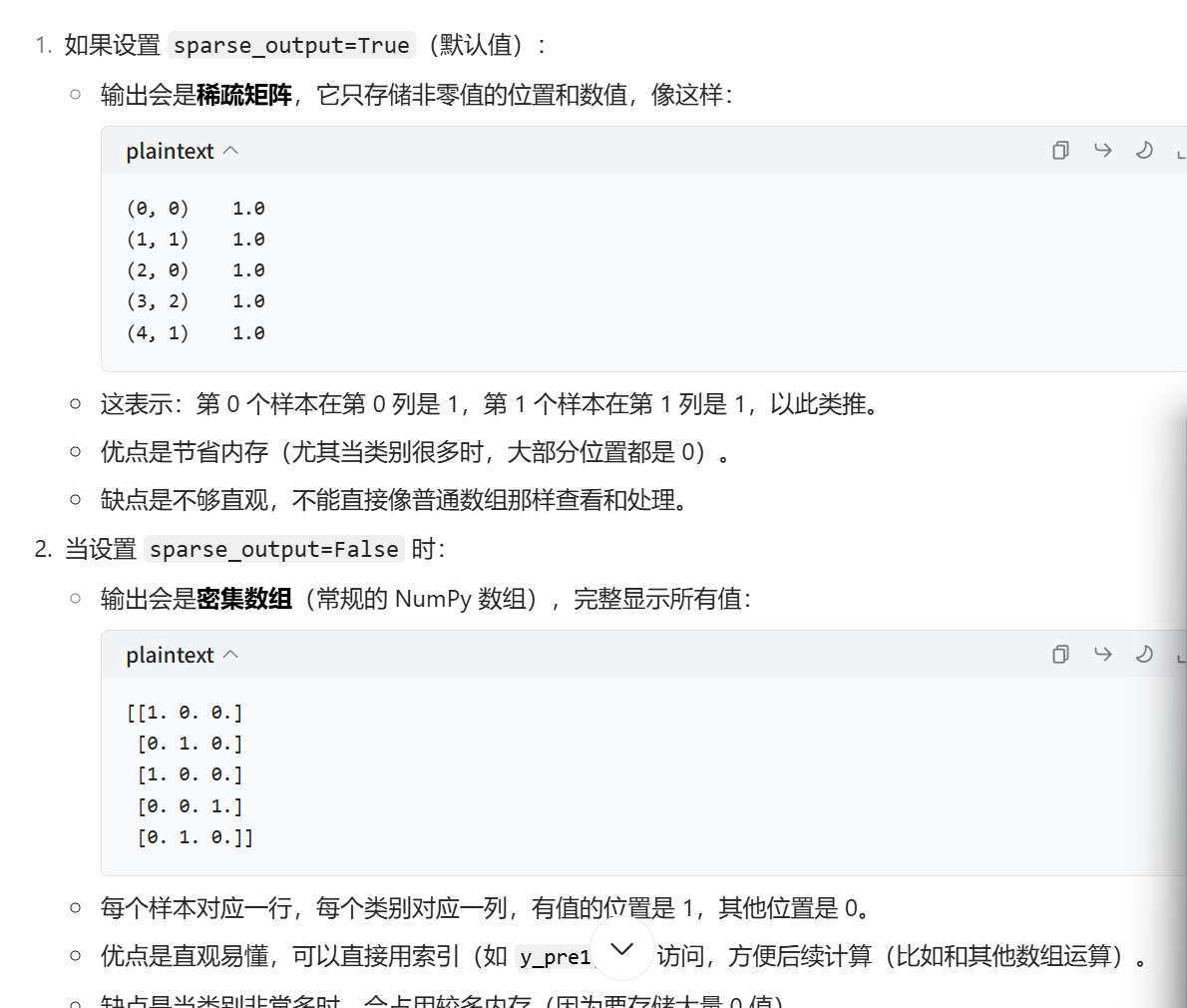
sparse_output=False：设置输出为密集数组（而非稀疏矩阵），这样得到的编码结果是常规的 NumPy 数组，更直观易处理

#logloss模型评估
from sklearn.metrics import log_loss
log_loss(y_test1,y_pre1,normalize=True)

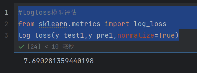
这样就求出来了
可以把logloss变小呢

#通过预测值，改变预测值的输出模式，让输出结果为百分占比，降低logloss
y_pre_proba=rf.predict_proba(x_test)
y_pre_proba

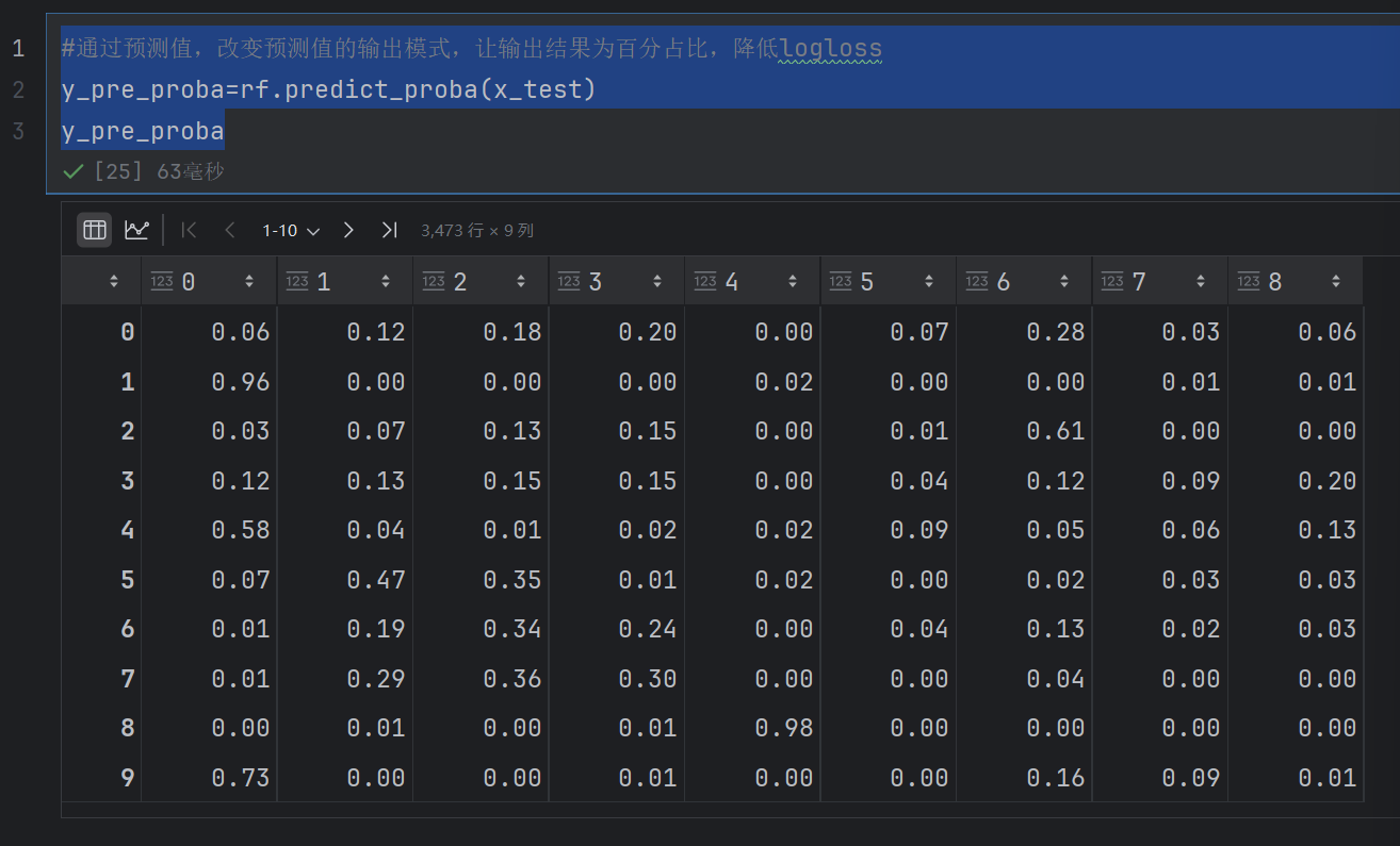
这个就是预测出现每个类别的可能性是多少
就不是直接预测可能是哪个类别，然后预测是每个类别的可能性是多少

log_loss(y_test1,y_pre_proba,normalize=True)

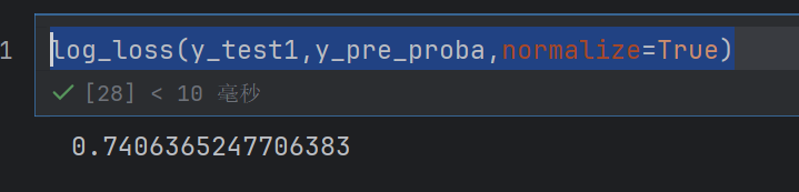
这个logloss直接就变成零点几了

4.4 模型调优

#模型调优-->超参数
##确定最优的n_estimators
tuned_parameters = range(10,200,10)
#创建添加accuracy的numpy
accuracy_t = np.zeros(len(tuned_parameters))
#创建添加error的numpy
error_t = np.zeros(len(tuned_parameters))
#调优过程实现
for i,n_estimators in enumerate(tuned_parameters):rf2 = RandomForestClassifier(n_estimators=n_estimators,max_depth=10,max_features=10,min_samples_leaf=10,random_state=0,n_jobs=-1,oob_score=True)rf2.fit(x_train,y_train)accuracy_t[i] = rf2.oob_score_y_pre=rf2.predict_proba(x_test)error_t[i]=log_loss(y_test1,y_pre,normalize=True)print(error_t)

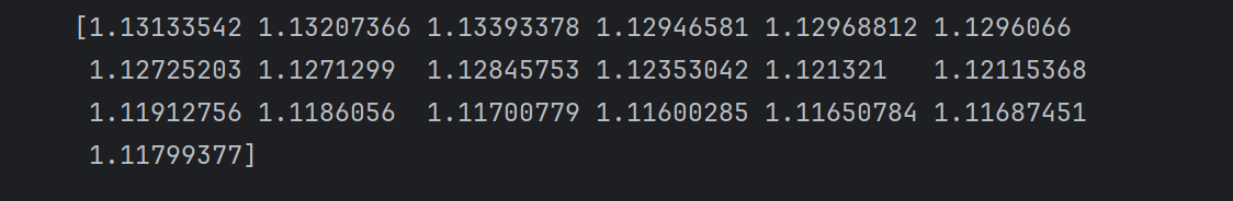
我们直接看最后的输出，发现logloss是一直在变小的

#优化结果过程可视化
fig,axes=plt.subplots(nrows=1,ncols=2,figsize=(20,4),dpi=100)
axes[0].plot(tuned_parameters,error_t)
axes[0].set_xlabel("n_estimators")
axes[0].set_ylabel("error_t")
axes[0].grid(True)
axes[1].plot(tuned_parameters,accuracy_t)
axes[1].set_xlabel("n_estimators")
axes[1].set_ylabel("accuracy_t")
axes[1].grid(True)
plt.show()

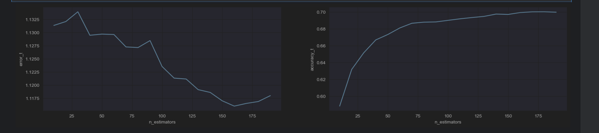
所以经过图像展示，发现n_estimators=175就和合适，logloss就很小，然后accuracy_t很高

#模型调优-->超参数
##确定最优的max_features
tuned_parameters = range(5,40,5)
#创建添加accuracy的numpy
accuracy_t = np.zeros(len(tuned_parameters))
#创建添加error的numpy
error_t = np.zeros(len(tuned_parameters))
#调优过程实现
for i,n_estimators in enumerate(tuned_parameters):rf2 = RandomForestClassifier(n_estimators=175,max_depth=10,max_features=n_estimators,min_samples_leaf=10,random_state=0,n_jobs=-1,oob_score=True)rf2.fit(x_train,y_train)accuracy_t[i] = rf2.oob_score_y_pre=rf2.predict_proba(x_test)error_t[i]=log_loss(y_test1,y_pre,normalize=True)print(error_t)

#优化结果过程可视化
fig,axes=plt.subplots(nrows=1,ncols=2,figsize=(20,4),dpi=100)
axes[0].plot(tuned_parameters,error_t)
axes[0].set_xlabel("max_features")
axes[0].set_ylabel("error_t")
axes[0].grid(True)
axes[1].plot(tuned_parameters,accuracy_t)
axes[1].set_xlabel("max_features")
axes[1].set_ylabel("accuracy_t")
axes[1].grid(True)
plt.show()

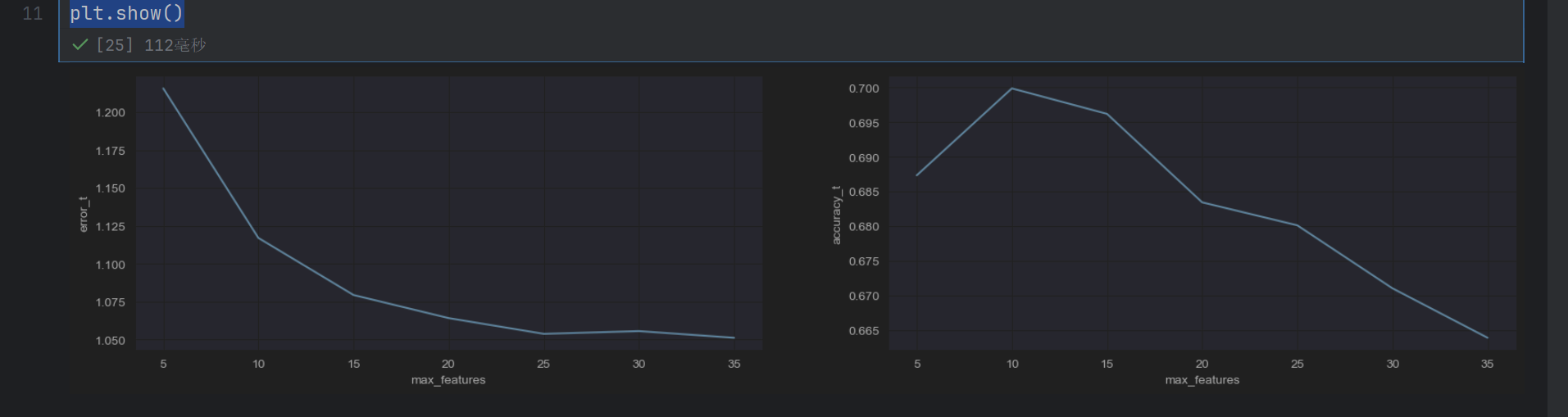
发现max_features=15的时候就很好了

#模型调优-->超参数
##确定最优的max_depth
tuned_parameters = range(10,100,10)
#创建添加accuracy的numpy
accuracy_t = np.zeros(len(tuned_parameters))
#创建添加error的numpy
error_t = np.zeros(len(tuned_parameters))
#调优过程实现
for i,n_estimators in enumerate(tuned_parameters):rf2 = RandomForestClassifier(n_estimators=175,max_depth=n_estimators,max_features=15,min_samples_leaf=10,random_state=0,n_jobs=-1,oob_score=True)rf2.fit(x_train,y_train)accuracy_t[i] = rf2.oob_score_y_pre=rf2.predict_proba(x_test)error_t[i]=log_loss(y_test1,y_pre,normalize=True)print(error_t)

#优化结果过程可视化
fig,axes=plt.subplots(nrows=1,ncols=2,figsize=(20,4),dpi=100)
axes[0].plot(tuned_parameters,error_t)
axes[0].set_xlabel("max_depth")
axes[0].set_ylabel("error_t")
axes[0].grid(True)
axes[1].plot(tuned_parameters,accuracy_t)
axes[1].set_xlabel("max_depth")
axes[1].set_ylabel("accuracy_t")
axes[1].grid(True)
plt.show()

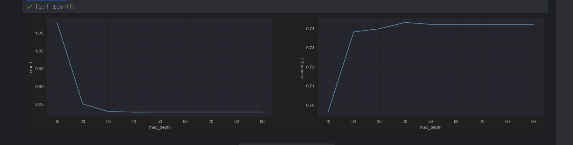
发现max_depth=30刚刚好

min_samples_leaf 是一个重要的超参数，用于控制决策树叶子节点的最小样本数量

当 min_samples_leaf=1 时，允许叶子节点只包含 1 个样本（最灵活但可能过拟合）
当 min_samples_leaf=10 时，要求每个叶子节点至少包含 10 个样本（更保守，不易过拟合）

#模型调优-->超参数
##确定最优的min_samples_leaf
tuned_parameters = range(1,10,2)
#创建添加accuracy的numpy
accuracy_t = np.zeros(len(tuned_parameters))
#创建添加error的numpy
error_t = np.zeros(len(tuned_parameters))
#调优过程实现
for i,n_estimators in enumerate(tuned_parameters):rf2 = RandomForestClassifier(n_estimators=175,max_depth=30,max_features=15,min_samples_leaf=n_estimators,random_state=0,n_jobs=-1,oob_score=True)rf2.fit(x_train,y_train)accuracy_t[i] = rf2.oob_score_y_pre=rf2.predict_proba(x_test)error_t[i]=log_loss(y_test1,y_pre,normalize=True)print(error_t)

#优化结果过程可视化
fig,axes=plt.subplots(nrows=1,ncols=2,figsize=(20,4),dpi=100)
axes[0].plot(tuned_parameters,error_t)
axes[0].set_xlabel("min_samples_leaf")
axes[0].set_ylabel("error_t")
axes[0].grid(True)
axes[1].plot(tuned_parameters,accuracy_t)
axes[1].set_xlabel("min_samples_leaf")
axes[1].set_ylabel("accuracy_t")
axes[1].grid(True)
plt.show()

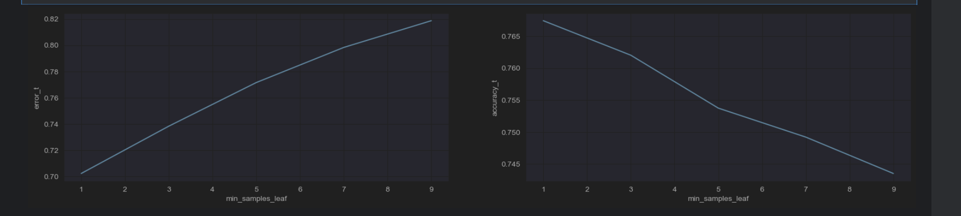
所以min_samples_leaf=1

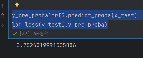
rf3 = RandomForestClassifier(n_estimators=175,max_depth=30,max_features=15,min_samples_leaf=1,random_state=0,n_jobs=-1,oob_score=True)
rf3.fit(x_train,y_train)

y_pre_proba1=rf3.predict_proba(x_test)
log_loss(y_test1,y_pre_proba)

4.5 生成提交数据

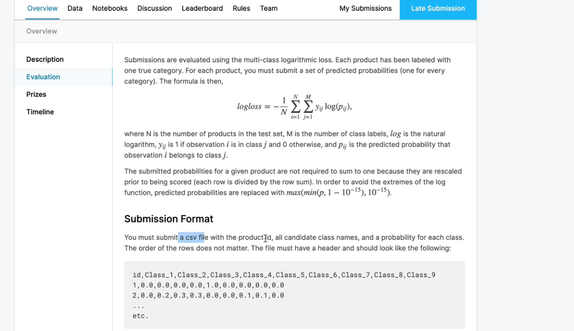
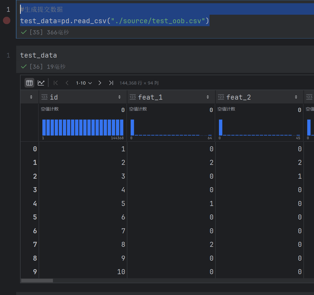
#生成提交数据
test_data=pd.read_csv("./source/test_oob.csv")

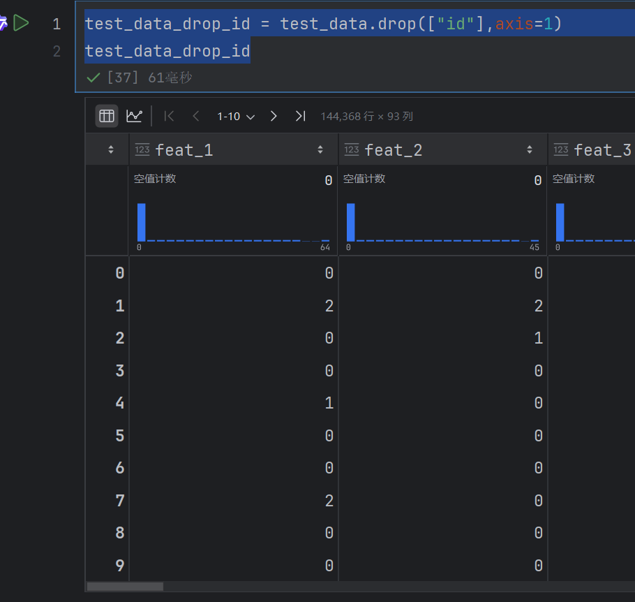
test_data_drop_id = test_data.drop(["id"],axis=1)
test_data_drop_id

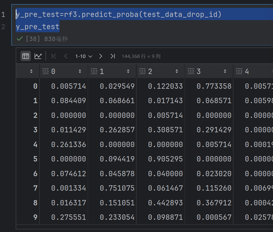
y_pre_test=rf3.predict_proba(test_data_drop_id)
y_pre_test

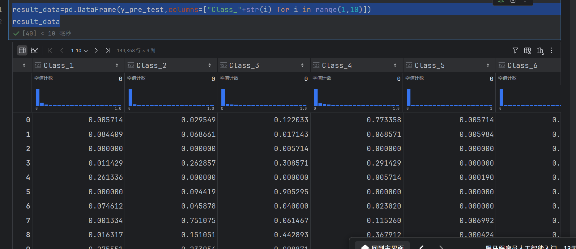
result_data=pd.DataFrame(y_pre_test,columns=["Class_"+str(i) for i in range(1,10)])
result_data

result_data.insert(loc=0,column="id",value=test_data["id"])
result_data

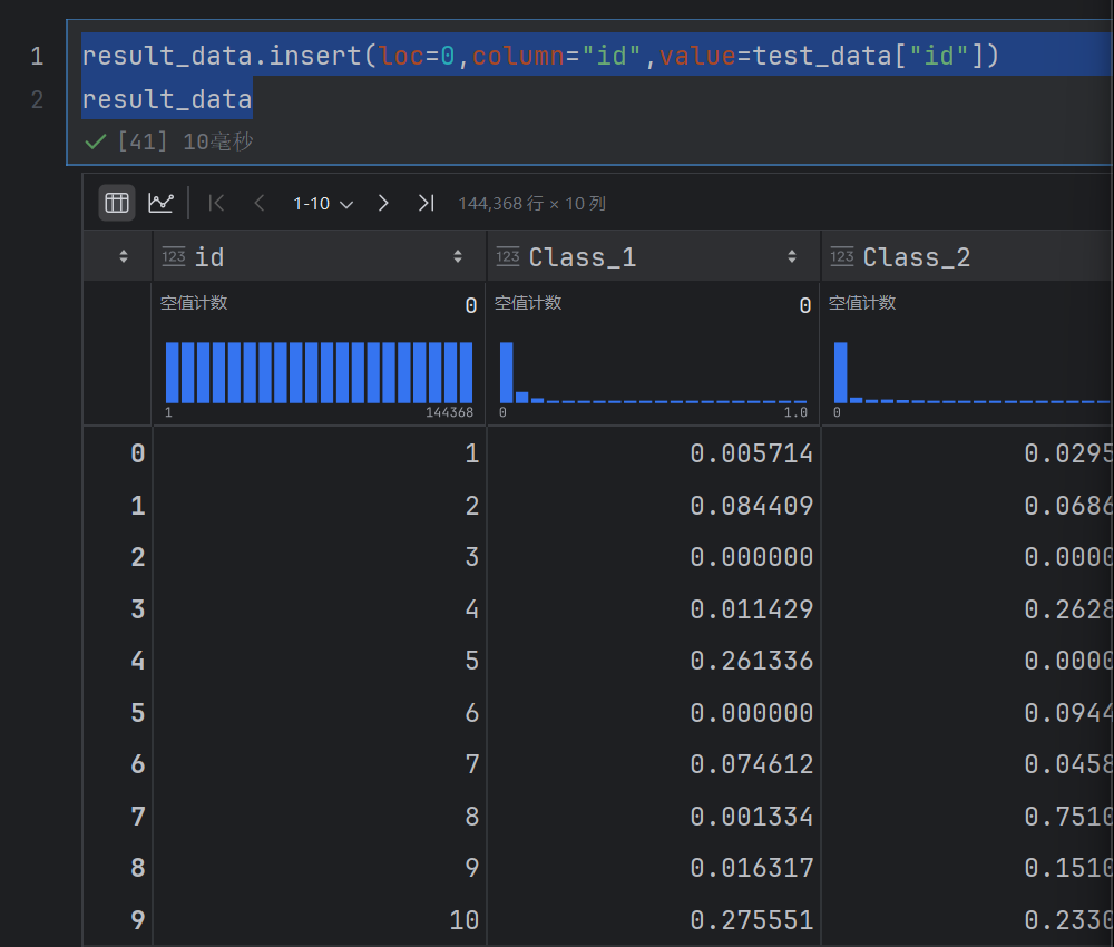
然后就可以存储为csv文件了

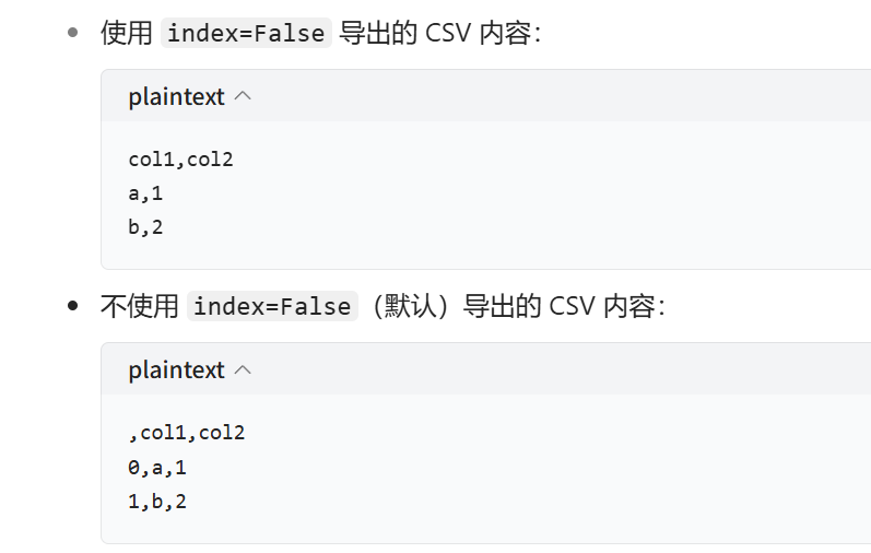
result_data.to_csv("./source/otto_result.csv",index=False)

当 index=False 时：导出 CSV 文件时不会包含 DataFrame 的索引列，只保存数据列

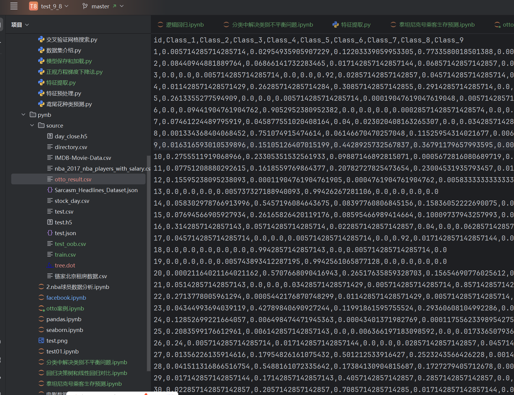
注意这里的id不是索引

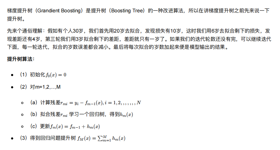
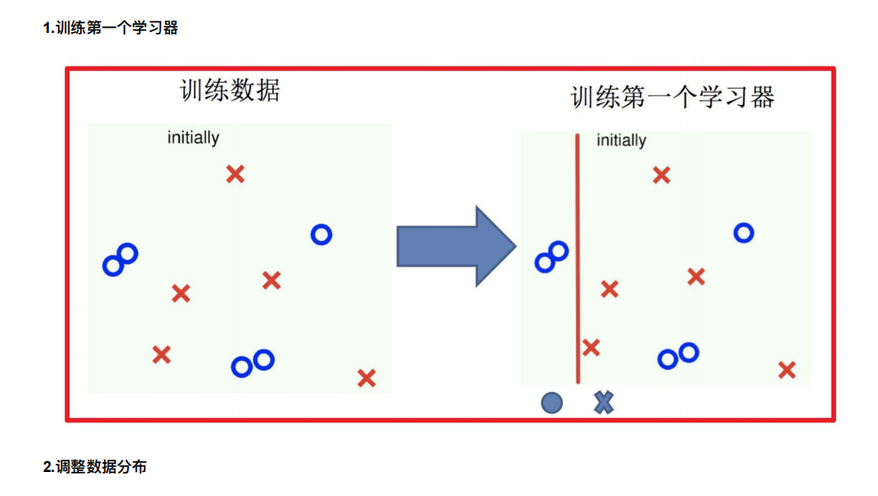
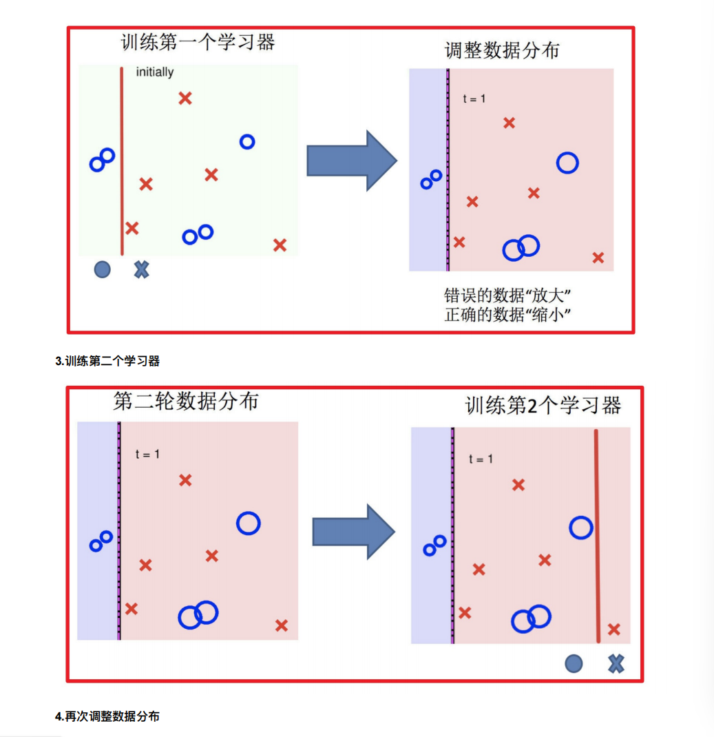
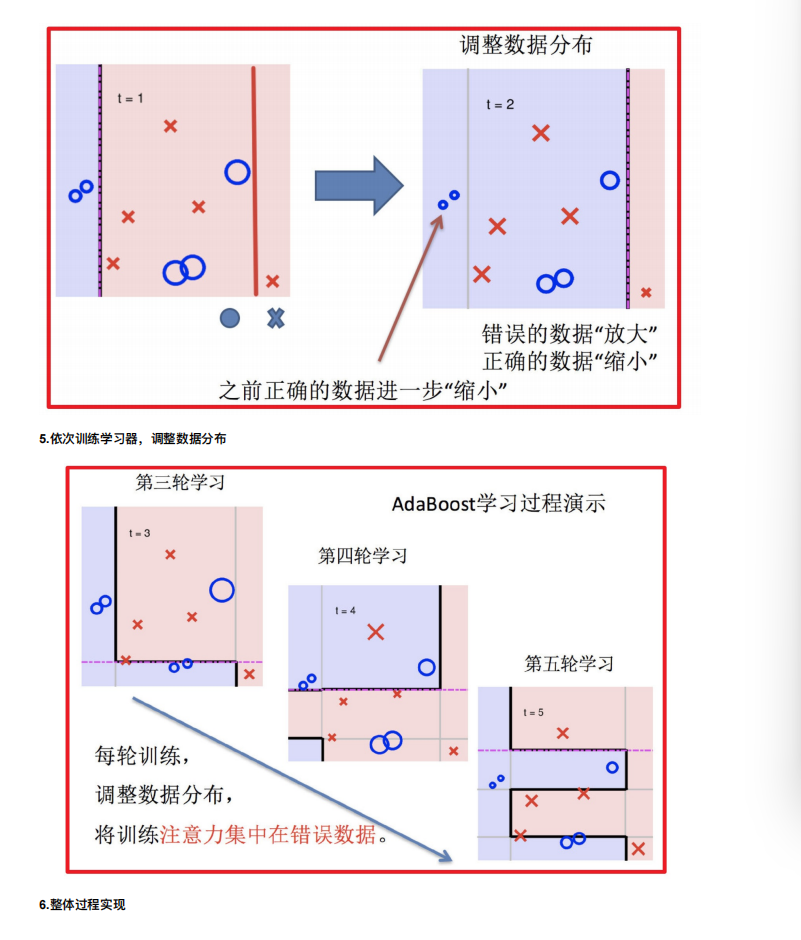
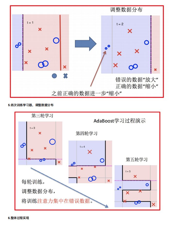
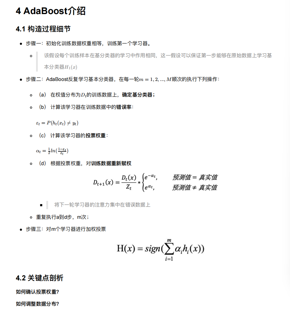
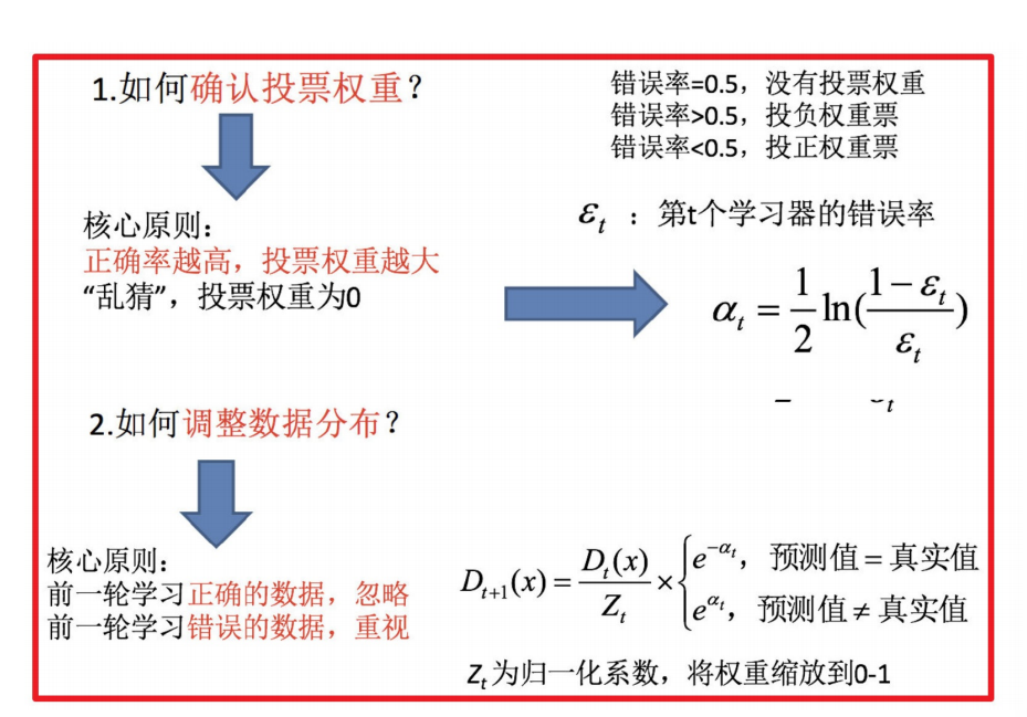
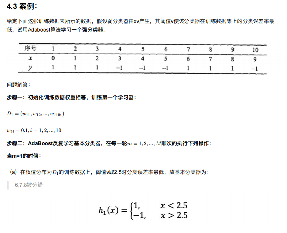
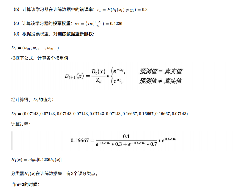
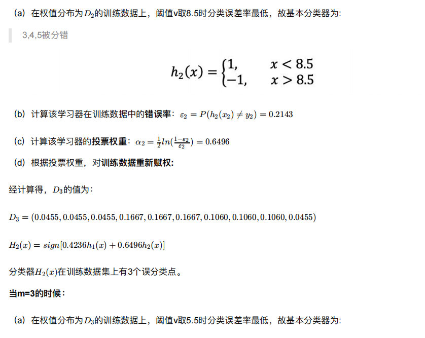
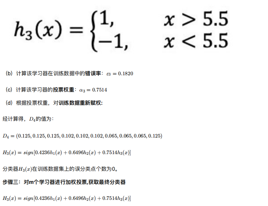
4. Boosting

随着学习的积累从弱到强
简⽽⾔之：每新加⼊⼀个弱学习器，整体能⼒就会得到提升

代表算法：Adaboost，GBDT，XGBoost，LightGBM

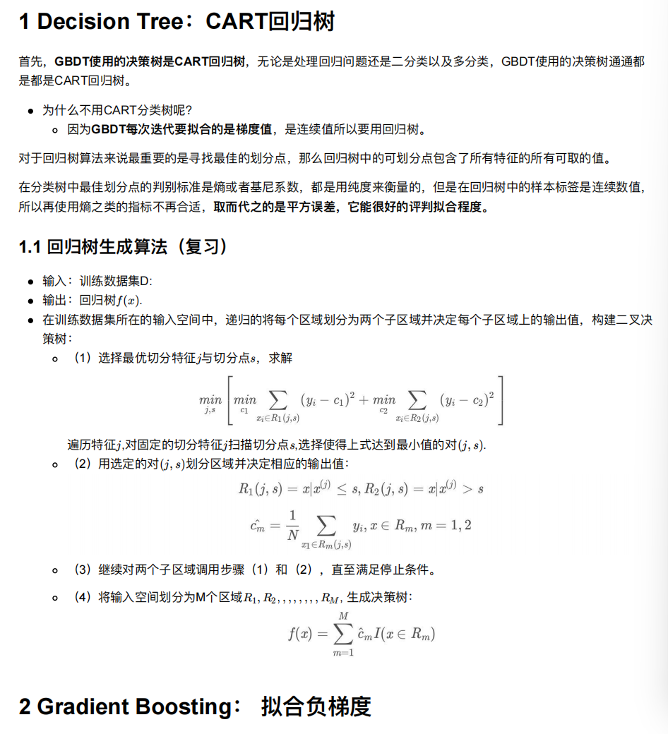
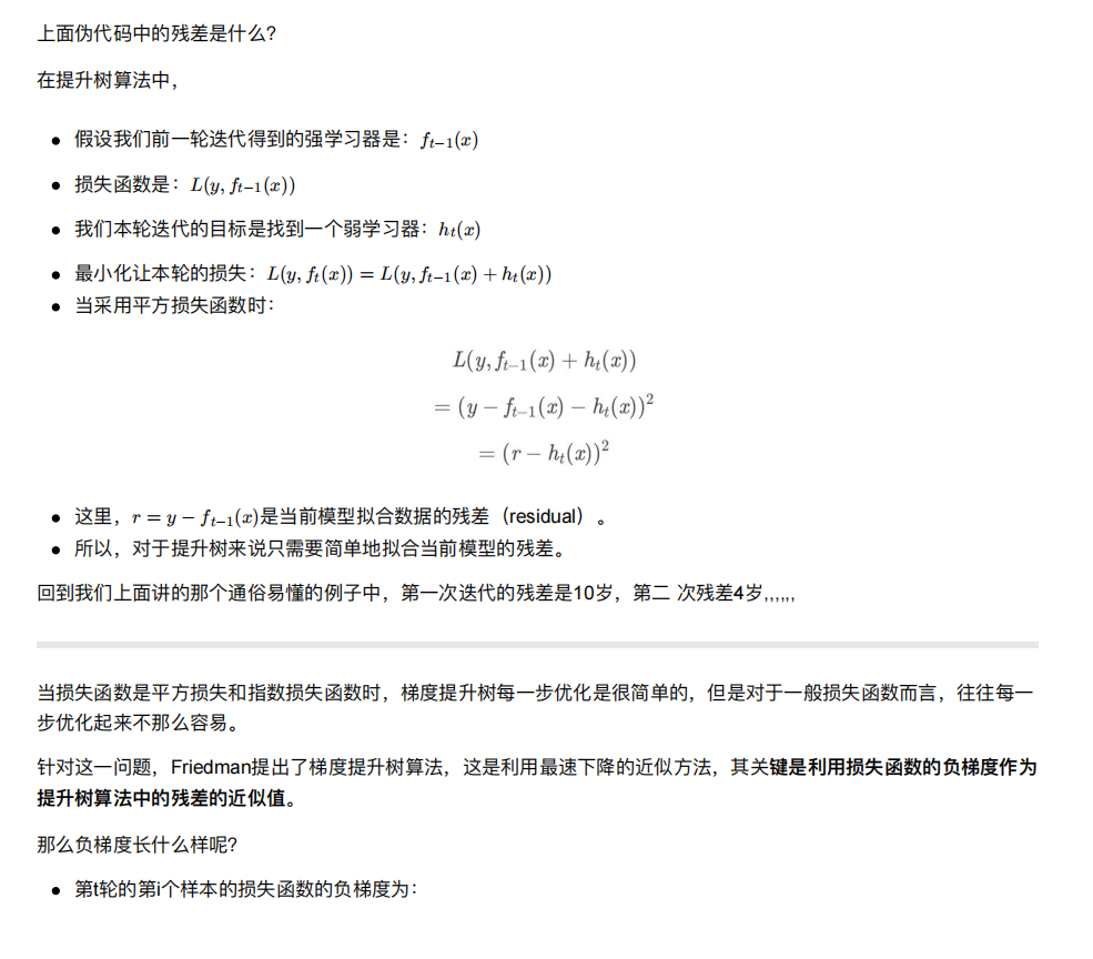
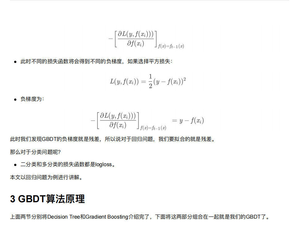
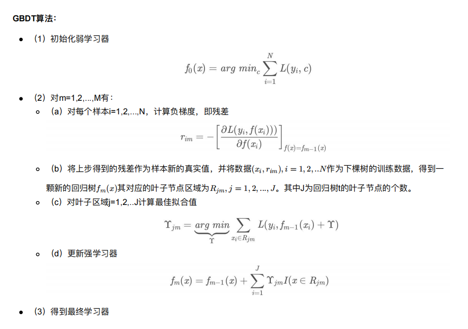
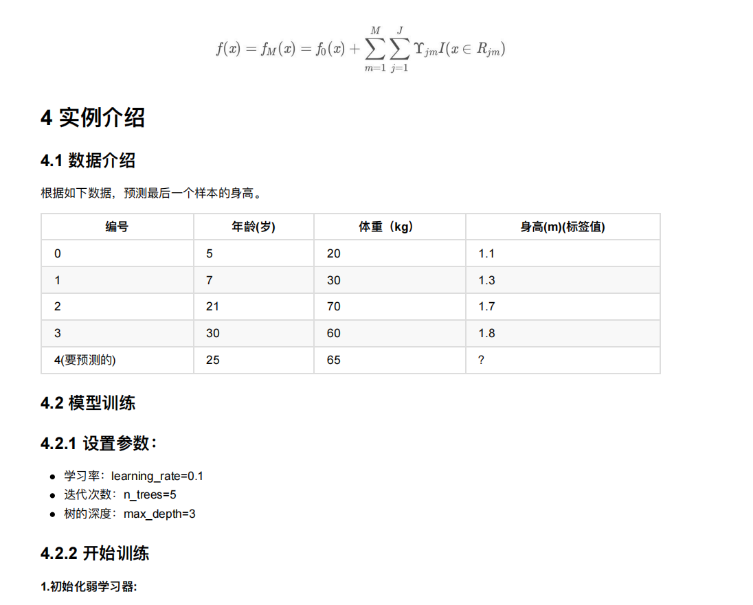
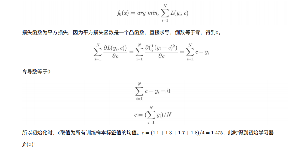
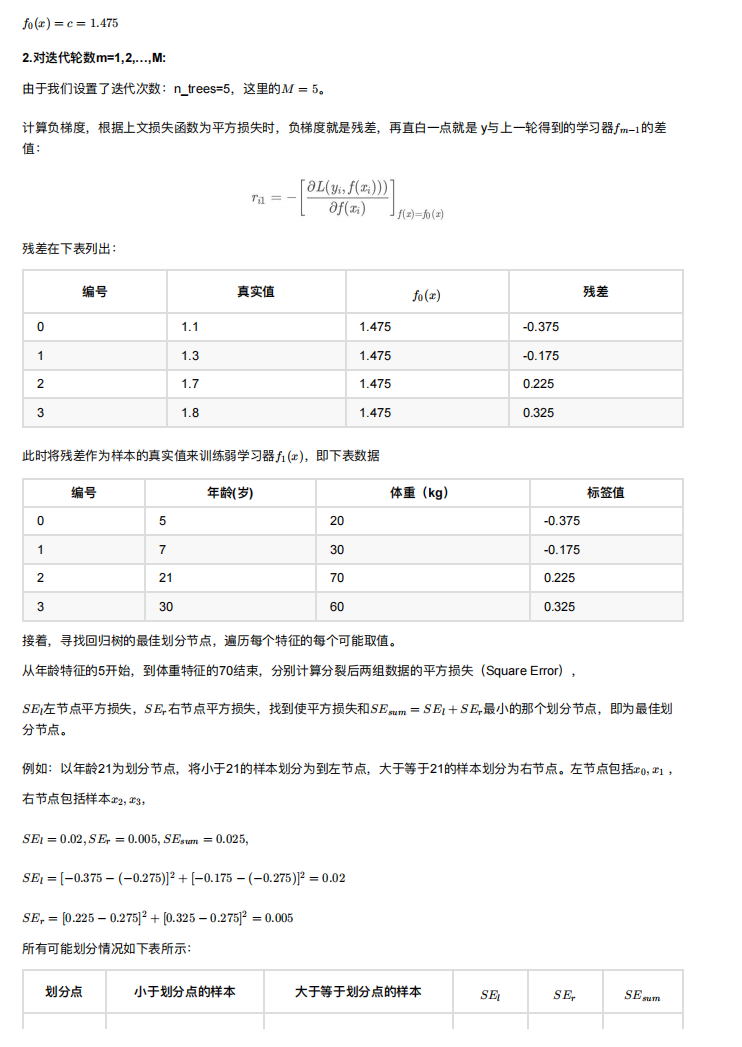
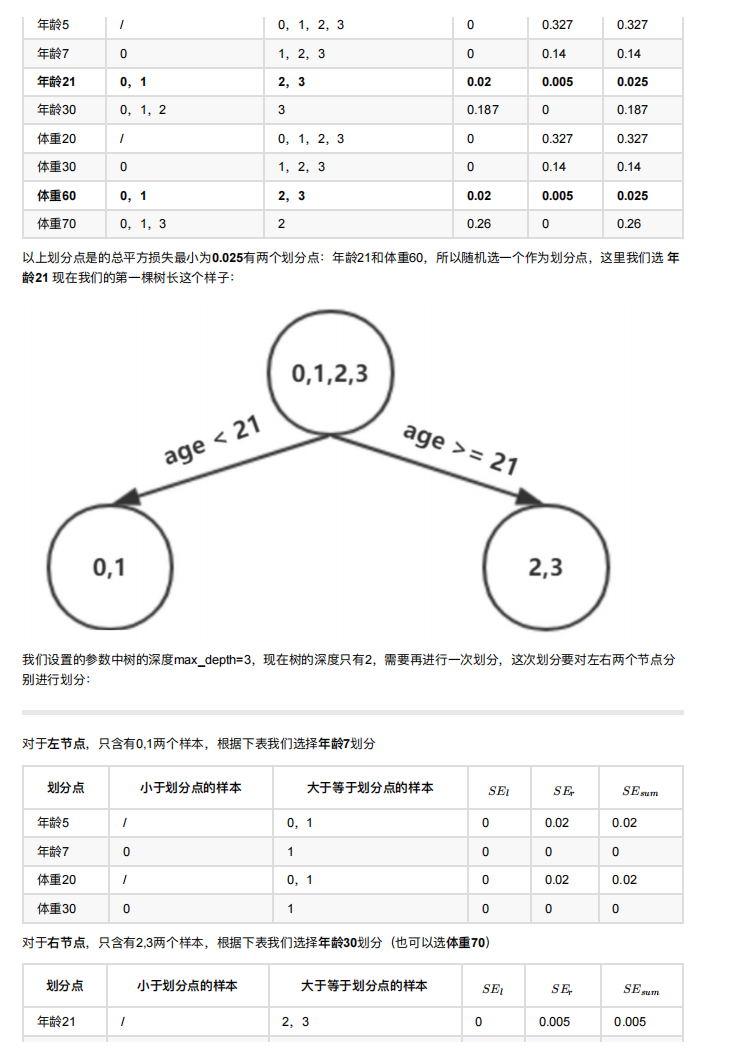
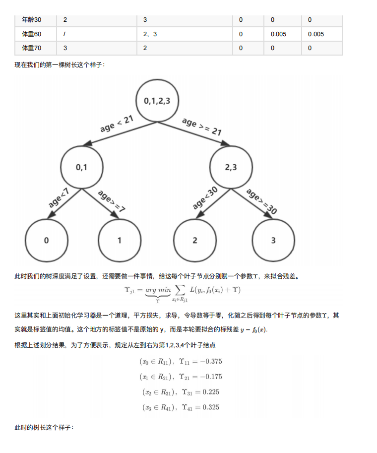
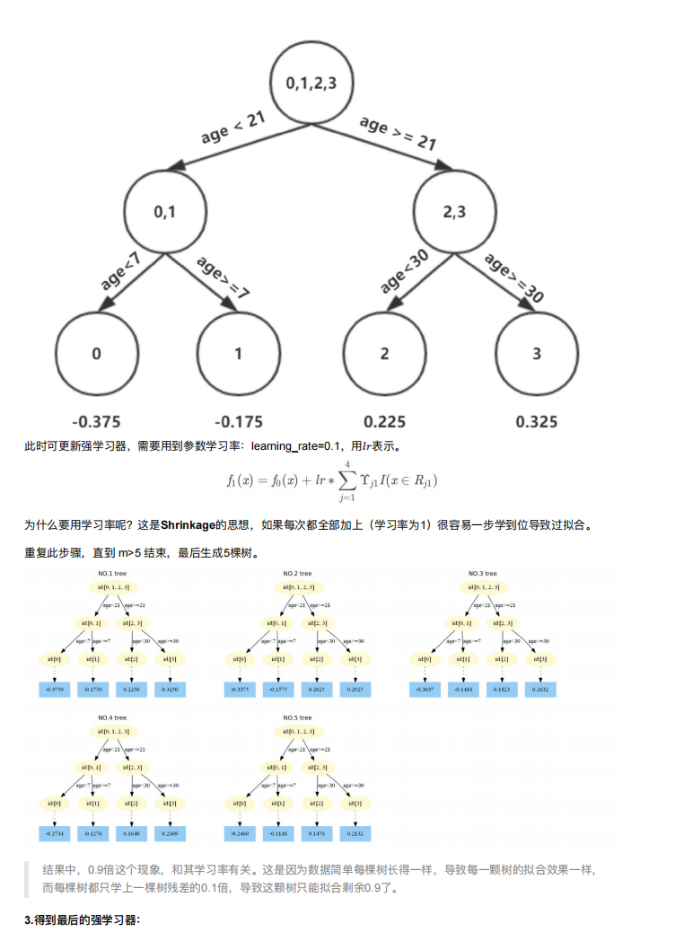
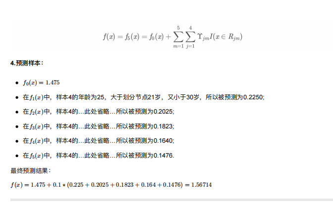
5. GBDT介绍

GBDT 的全称是 Gradient Boosting Decision Tree，梯度提升树，在传统机器学习算法中，GBDT算的上TOP3的算法。
想要理解GBDT的真正意义，那就必须理解GBDT中的Gradient Boosting 和Decision Tree分别是什么？

总结13.03