Field II 超声成像仿真 --2-CPWC (Coherent Plane-Wave Compounding)
个人记录
CPWC(Coherent Plane-Wave Compounding)——实现主干 + 工作流
一、实现主干(模块化视角)
1. 初始化环境
清理工作区,加载 USTB 路径
设置基本常量:声速
c0、采样频率fs、时间步长dt
2.Field II 初始化
field_init(0)设置声速、采样率、单元形状
field_init(0);
set_field('c',c0);              % Speed of sound [m/s]
set_field('fs',fs);             % Sampling frequency [Hz]
set_field('use_rectangles',1);  % use rectangular elements
3.探头建模 (Probe)
使用
uff.linear_array()定义 L11-4v 128 阵元探头参数设置中心频率
f0、波长lambda、阵元宽高、间距pitch、数量N等
4.脉冲建模 (Pulse)
使用高斯脉冲 + 方波激励生成发射脉冲
计算发射/接收冲激响应,并绘制脉冲检查对称性
pulse = uff.pulse();
pulse.fractional_bandwidth = 0.65;        % probe bandwidth [1]
pulse.center_frequency = f0;
t0 = (-1/pulse.fractional_bandwidth/f0): dt : (1/pulse.fractional_bandwidth/f0);
impulse_response = gauspuls(t0, f0, pulse.fractional_bandwidth);
impulse_response = impulse_response-mean(impulse_response); % To get rid of DCte = (-pulse_duration/2/f0): dt : (pulse_duration/2/f0);
excitation = square(2*pi*f0*te+pi/2);
one_way_ir = conv(impulse_response,excitation);
two_way_ir = conv(one_way_ir,impulse_response);
lag = length(two_way_ir)/2+1;
5.
发射与接收孔径定义 (Aperture)
xdc_linear_array()建立发射/接收孔径设置激励、冲激响应、挡板、聚焦方式
6.平面波序列定义 (Plane Wave Sequence)
设置最大角度
alpha_max = atan(1/2/F_number)生成多个角度
alpha = linspace(-alpha_max, alpha_max, Na)
%% Define plane wave sequence
% Define the start_angle and number of angles
F_number = 1.7;
alpha_max = atan(1/2/F_number);
Na=15;                                      % number of plane waves
F=1;                                        % number of frames
alpha=linspace(-alpha_max,alpha_max,Na);    % vector of angles [rad]
7.
虚拟体模 (Phantom)
定义散射体点源的位置和幅值
8.数据存储预分配
CPW=zeros(cropat,probe.N,Na,F);cropat 决定采样截断长度(节省内存)
9.核心循环:CPWC 数据计算
xdc_apodization(Th,0,ones(1,probe.N)):发射 apod 矩阵(这里是矩形窗),0 表示时刻/状态编号。
xdc_times_focus(Th,0,probe.geometry(:,1)'.*sin(alpha(n))/c0):这是平面波发射延迟公式。probe.geometry(:,1)'取每个元的横坐标 xex_exe,延迟 = xesinα/c。注意probe.geometry必须有正确坐标(UFF probe 通常包含)。
Rh接收端不设置动态聚焦(xdc_focus_times(Rh, 0, zeros(1,probe.N))),以全阵元接收原始通道数据
calc_scat_multi(Th, Rh, point_position, point_amplitudes):Field II 返回
v:矩阵[Nsamples × Nelements](每个接收通道的时序),
t:时间向量[Nsamples × 1],单位秒,表示每个样点相对于 Field II 内部时间基准的时刻
%% Compute CPW signals
time_index=0;
disp('Field II: Computing CPW dataset');
wb = waitbar(0, 'Field II: Computing CPW dataset');
for f=1:Fwaitbar(0, wb, sprintf('Field II: Computing CPW dataset, frame %d',f));for n=1:Nawaitbar(n/Na, wb);disp(['Calculating angle ',num2str(n),' of ',num2str(Na)]);% transmit aperturexdc_apodization(Th,0,ones(1,probe.N));xdc_times_focus(Th,0,probe.geometry(:,1)'.*sin(alpha(n))/c0);% receive aperturexdc_apodization(Rh, 0, ones(1,probe.N));xdc_focus_times(Rh, 0, zeros(1,probe.N));% do calculation[v,t]=calc_scat_multi(Th, Rh, point_position, point_amplitudes);% build the datasetCPW(1:size(v,1),:,n,f)=v;% Save transmit sequenceseq(n)=uff.wave();seq(n).probe=probe;seq(n).source.azimuth=alpha(n);seq(n).source.distance=Inf;seq(n).sound_speed=c0;seq(n).delay = -lag*dt+t;end
end
close(wb);
10.Channel Data (UFF) 封装
11. Scan / Pipeline / DAS + Coherent Compounding
sca = uff.linear_scan('x_axis',linspace(-10e-3,10e-3,256).', 'z_axis', linspace(5e-3,20e-3,256).');pipe = pipeline();
pipe.channel_data = channel_data;
pipe.scan = sca;
pipe.receive_apodization.window = uff.window.tukey25;
pipe.receive_apodization.f_number = F_number;b_data = pipe.go({midprocess.das() postprocess.coherent_compounding()});
b_data.plot();
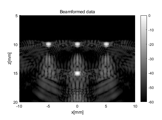
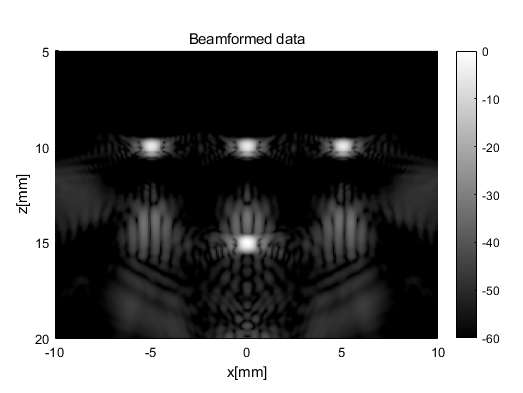
仿真结果:
'realtime'