当前位置：首页 > news >正文

随机森林模型：基于天气数据集的分类任务全流程解析

news 2025/9/16 12:44:58

随机森林（Random Forest, RF）是机器学习中经典的集成学习算法，通过组合多棵决策树的预测结果提升模型泛化能力，兼具 “高准确率” 与 “强抗过拟合能力”。本文以人工合成的天气数据集为案例，从数据加载、预处理、探索性分析到随机森林模型构建、评估与特征重要性解读，完整拆解随机森林在分类任务中的应用流程。

一、项目背景与核心目标

1. 数据集介绍

本次使用的天气分类数据集（weather_classification_data.csv） 包含 13200 条样本，每条样本含 11 个字段，涵盖气象观测指标与天气类型标签，具体字段含义如下：

列名	中文解释	单位	数据类型	备注
Temperature	温度	摄氏度	数值型（float64）	范围 - 25°C~109°C，含极端异常值
Humidity	湿度	%	数值型（int64）	合理范围 0%~100%，部分数据超上限
Wind Speed	风速	km/h	数值型（float64）	含台风等极端高风速数据
Precipitation (%)	降水量	%	数值型（float64）	部分数据超 100%，需异常值处理
Cloud Cover	云量	-	分类型（object）	取值：clear、cloudy、overcast、partly cloudy
Atmospheric Pressure	气压	hPa	数值型（float64）	标准范围 990~1020 hPa
UV Index	紫外线指数	-	数值型（int64）	反映紫外线强度，0~14
Season	季节	-	分类型（object）	取值：Winter、Spring、Summer、Autumn
Visibility (km)	能见度	km	数值型（float64）	受雾霾、雨雪影响较大
Location	地点	-	分类型（object）	取值：inland（内陆）、mountain（山区）、coastal（沿海）
Weather Type	天气类型	-	分类型（object）	目标变量，取值：Rainy（雨天）、Cloudy（阴天）、Sunny（晴天）、Snowy（雪天）

2. 核心目标

构建随机森林分类模型，基于 10 个气象特征预测天气类型（4 分类任务）；
掌握数据预处理（异常值处理、分类型特征编码）的关键步骤；
通过特征重要性分析，识别影响天气类型的核心气象指标；
理解决随机森林的抗过拟合机制，对比单棵决策树与集成模型的优势。

二、技术工具与环境准备

编程语言：Python 3.9

核心库说明：

库名	核心用途
`pandas/numpy`	数据加载、结构化处理与数值计算
`matplotlib/seaborn`	数据可视化（箱线图、直方图、特征重要性图）
`sklearn.ensemble`	随机森林模型实现（`RandomForestClassifier`）
`sklearn.preprocessing`	分类型特征编码（`LabelEncoder`）
`sklearn.model_selection`	数据集拆分（训练集 / 测试集）
`sklearn.metrics`	分类模型评估（准确率、精确率、F1 值等）

三、随机森林核心原理铺垫

在实战前，先明确随机森林的核心逻辑，帮助理解后续代码设计：

1. 随机森林的 “随机” 体现在哪里

随机森林通过两种随机机制降低单棵决策树的过拟合风险，提升集成模型的稳定性：

样本随机（Bootstrap 抽样）：从训练集中有放回地随机抽取样本，为每棵决策树构建独立的训练集（如 1000 条样本的数据集，每次抽 1000 条，允许重复）；
特征随机：每棵决策树分裂节点时，仅从全部特征的子集中选择最优分裂特征（如 10 个特征，每次随机选 5 个）。

2. 随机森林的预测逻辑（分类任务）

单棵决策树：对输入样本输出一个类别预测；
集成预测：通过多数投票制确定最终类别（如 100 棵树中 60 棵预测 “晴天”，则最终结果为 “晴天”）。

3. 随机森林 vs 单棵决策树

对比维度	单棵决策树	随机森林
过拟合风险	高（易过度学习训练集噪声）	低（随机机制 + 多树集成降低方差）
准确率	中等（对数据细节敏感）	高（综合多树优势，鲁棒性强）
可解释性	强（树结构清晰，可直观解读）	弱（多树集成，难以追溯单个预测的决策路径）
计算成本	低（仅训练一棵数）	高（训练多棵树，预测时需遍历所有树）

四、实战：随机森林天气分类模型

1. 导入依赖库与环境配置

首先导入所需库，并配置中文显示（避免可视化中出现乱码）：

# 数据处理库
import pandas as pd
import numpy as np
# 可视化库
import seaborn as sns
import matplotlib.pyplot as plt
# 模型与工具库
from sklearn.ensemble import RandomForestClassifier
from sklearn.model_selection import train_test_split
from sklearn.preprocessing import LabelEncoder
from sklearn.metrics import accuracy_score, precision_score, recall_score, f1_score
# 其他配置
import warnings
warnings.filterwarnings('ignore')  # 忽略警告信息
plt.rcParams['font.sans-serif'] = ['SimHei']  # 显示中文
plt.rcParams['axes.unicode_minus'] = False  # 显示负号

2. 加载并初步探索数据集

通过本地路径加载 CSV 文件，查看数据基本结构、缺失值与统计特征：

# 加载数据（需替换为你的本地文件路径）
weather_data = pd.read_csv(r"D:\Desktop\CC是小陈\Machine Learning\weather_classification_data.csv")# 1. 查看前5行数据
print("=== 数据集前5行预览 ===")
print(weather_data.head())# 2. 查看数据基本信息（维度、数据类型、非空值）
print("\n=== 数据集基本信息 ===")
print(weather_data.info())
# 输出：13200条样本，11列（5个float、2个int、4个object），无缺失值# 3. 查看数值型特征的统计描述
print("\n=== 数值型特征统计描述 ===")
print(weather_data.describe())
# 关键发现：温度最大值109°C（异常）、湿度最大值109%（超上限）、降水量最大值109%（超上限）# 4. 检查缺失值
print("\n=== 各列缺失值数量 ===")
print(weather_data.isnull().sum())
# 输出：所有列缺失值均为0，数据完整性良好

初步探索结论

数据集无缺失值，无需缺失值填充；
数值型特征存在异常值（如温度 109°C、湿度 109%），需后续处理；
存在 4 个分类型特征（Cloud Cover、Season、Location、Weather Type），需编码为数值型才能输入模型。

3. 数据预处理：异常值处理与特征编码

数据预处理是随机森林模型性能的关键，需解决 “异常值干扰” 与 “分类型特征无法输入” 两个核心问题：

（1）异常值检测与处理

通过箱线图可视化数值型特征的分布，识别异常值，再根据业务逻辑删除不合理数据：

# 定义数值型特征与中文映射（用于可视化标签）
feature_map = {'Temperature': '温度','Humidity': '湿度百分比','Wind Speed': '风速','Precipitation (%)': '降水量百分比','Atmospheric Pressure': '大气压力','UV Index': '紫外线指数','Visibility (km)': '能见度'
}# 绘制箱线图，检测异常值
plt.figure(figsize=(15, 10))
for i, (col, col_name) in enumerate(feature_map.items(), 1):plt.subplot(2, 4, i)  # 2行4列子图sns.boxplot(y=weather_data[col], color='#1f77b4')plt.title(f'{col_name}的箱线图', fontsize=12)plt.ylabel('数值', fontsize=10)plt.grid(linestyle='--', alpha=0.2)
plt.tight_layout()  # 自动调整子图间距
plt.show()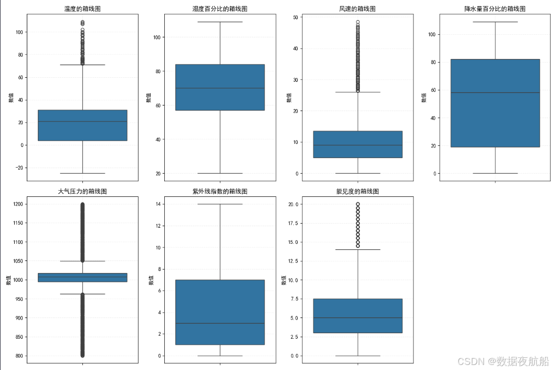

异常值判定逻辑（基于业务常识）

温度：超过 60°C 为异常（地球极端高温约 56.7°C）；
湿度 / 降水量：超过 100% 为异常（百分比指标上限为 100%）；
风速 / 气压 / 能见度：高值可能对应台风、高海拔等合理场景，暂不处理。

# 统计异常值数量与占比
print("=== 异常值统计 ===")
temp_abnormal = weather_data[weather_data['Temperature'] > 60].shape[0]
humidity_abnormal = weather_data[weather_data['Humidity'] > 100].shape[0]
precip_abnormal = weather_data[weather_data['Precipitation (%)'] > 100].shape[0]print(f"温度>60°C：{temp_abnormal}条（{temp_abnormal/len(weather_data)*100:.2f}%）")
print(f"湿度>100%：{humidity_abnormal}条（{humidity_abnormal/len(weather_data)*100:.2f}%）")
print(f"降水量>100%：{precip_abnormal}条（{precip_abnormal/len(weather_data)*100:.2f}%）")# 删除异常值（异常值占比<4%，删除对数据量影响小）
print(f"\n删除前数据量：{weather_data.shape[0]}条")
weather_data = weather_data[(weather_data['Temperature'] <= 60) & (weather_data['Humidity'] <= 100) & (weather_data['Precipitation (%)'] <= 100)
]
print(f"删除后数据量：{weather_data.shape[0]}条")
# 输出：删除后剩余12360条样本，保留93.6%的数据

（2）分类型特征编码（LabelEncoder）

随机森林模型仅接受数值型输入，需将分类型特征（如 “Cloud Cover” 的 “clear”“cloudy”）编码为整数（0、1、2 等）：

# 定义需编码的分类型特征
categorical_cols = ['Cloud Cover', 'Season', 'Location', 'Weather Type']# 创建LabelEncoder字典，保存每个特征的编码映射（便于后续解读）
label_encoders = {}
new_data = weather_data.copy()  # 复制数据，避免修改原数据集# 遍历特征，逐一编码
for col in categorical_cols:le = LabelEncoder()new_data[col] = le.fit_transform(new_data[col])  # 编码为0、1、2...label_encoders[col] = le  # 保存编码映射# 打印编码结果（便于后续解读预测结果）
print("\n=== 分类型特征编码映射 ===")
for col, le in label_encoders.items():print(f"\n{col}编码映射：")for idx, label in enumerate(le.classes_):print(f"  {label} → {idx}")

4. 探索性数据分析（EDA）：理解数据分布

通过可视化进一步分析数据特征与目标变量的关系，为模型结果解读做铺垫：

# 设置画布大小（20×15英寸，确保子图清晰）
plt.figure(figsize=(20, 15))# 1. 温度分布（直方图+核密度估计）
plt.subplot(3, 4, 1)
sns.histplot(new_data['Temperature'], kde=True, bins=20, color='#ff7f0e')
plt.title('温度分布', fontsize=12)
plt.xlabel('温度（°C）')
plt.ylabel('频次')# 2. 湿度分布（箱线图）
plt.subplot(3, 4, 2)
sns.boxplot(y=new_data['Humidity'], color='#2ca02c')
plt.title('湿度分布', fontsize=12)
plt.ylabel('湿度（%）')# 3. 风速分布（直方图）
plt.subplot(3, 4, 3)
sns.histplot(new_data['Wind Speed'], kde=True, bins=20, color='#d62728')
plt.title('风速分布', fontsize=12)
plt.xlabel('风速（km/h）')
plt.ylabel('频次')# 4. 降水量分布（箱线图）
plt.subplot(3, 4, 4)
sns.boxplot(y=new_data['Precipitation (%)'], color='#9467bd')
plt.title('降水量分布', fontsize=12)
plt.ylabel('降水量（%）')# 5. 云量分布（计数图）
plt.subplot(3, 4, 5)
cloud_mapping = dict(enumerate(label_encoders['Cloud Cover'].classes_))  # 编码→原标签
sns.countplot(x=new_data['Cloud Cover'].map(cloud_mapping), color='#8c564b')
plt.title('云量分布', fontsize=12)
plt.xlabel('云量类型')
plt.ylabel('频次')
plt.xticks(rotation=45)  # 旋转标签，避免重叠# 6. 季节分布（饼图）
plt.subplot(3, 4, 8)
season_mapping = dict(enumerate(label_encoders['Season'].classes_))
season_counts = new_data['Season'].map(season_mapping).value_counts()
plt.pie(season_counts, labels=season_counts.index, autopct='%1.1f%%', startangle=140, colors=['#ff9999','#66b3ff','#99ff99','#ffcc99'])
plt.title('季节分布', fontsize=12)# 7. 天气类型分布（计数图，目标变量）
plt.subplot(3, 4, (11, 12))  # 跨两列显示
weather_mapping = dict(enumerate(label_encoders['Weather Type'].classes_))
sns.countplot(x=new_data['Weather Type'].map(weather_mapping), palette='Set2')
plt.title('天气类型分布（目标变量）', fontsize=12)
plt.xlabel('天气类型')
plt.ylabel('频次')plt.tight_layout()
plt.show()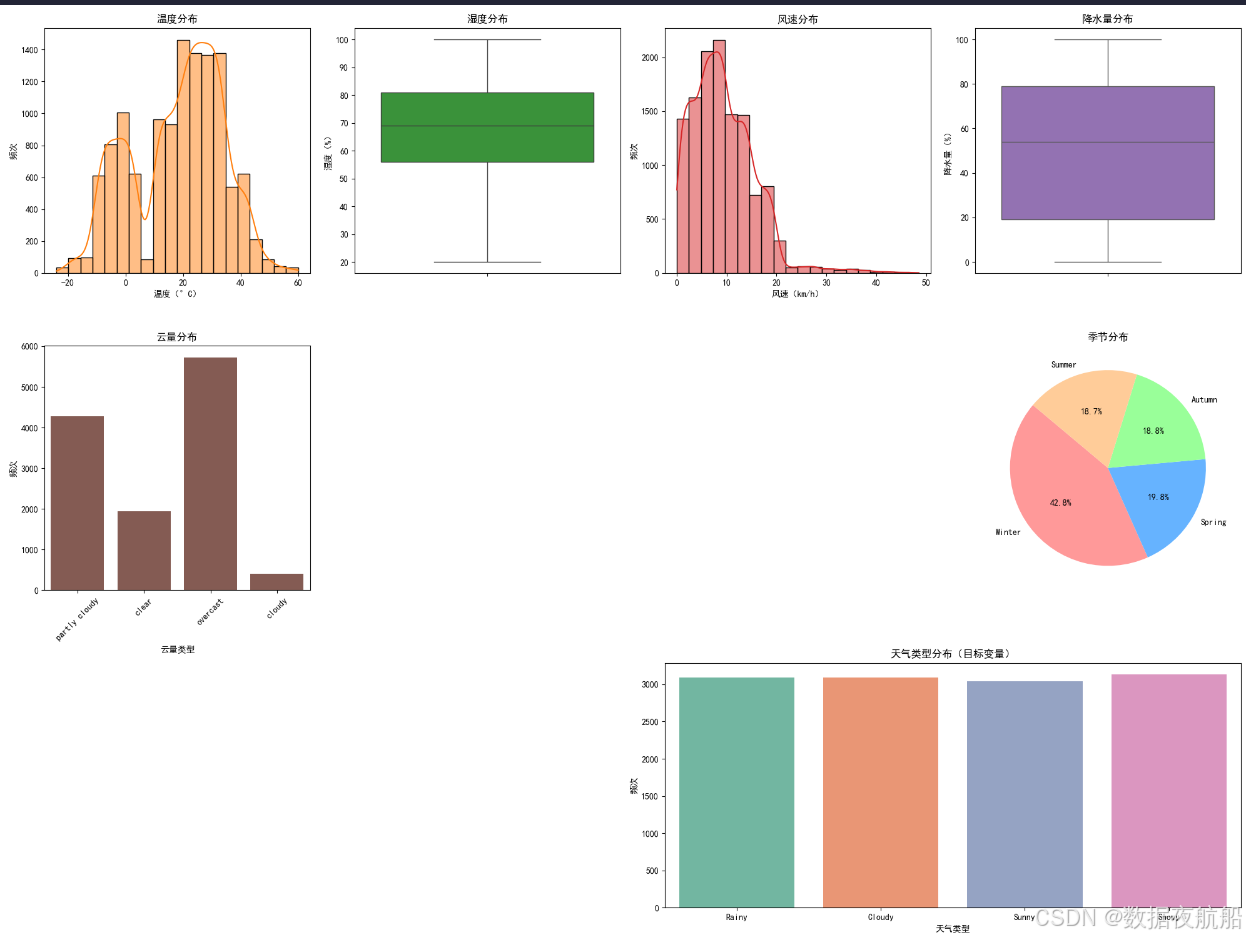

EDA 关键结论

温度：主要集中在 0°C~40°C，分布左偏（低温样本略多）；
湿度：多数在 50%~90%，分布对称；
天气类型：4 类分布较均匀（无明显类别不平衡），模型无需额外处理类别权重；
季节：冬季样本占比最高（约 30%），可能与数据采集地区气候相关。

5. 构建并训练随机森林模型

（1）拆分训练集与测试集

按 “7:3” 比例拆分数据集，确保模型泛化能力可评估：

# 提取特征矩阵X（删除目标变量Weather Type）与目标变量y
X = new_data.drop('Weather Type', axis=1)
y = new_data['Weather Type']# 拆分数据集：test_size=0.3（测试集30%），random_state=42（结果可复现）
X_train, X_test, y_train, y_test = train_test_split(X, y, test_size=0.3, random_state=42
)# 查看拆分后维度
print("=== 数据集拆分结果 ===")
print(f"训练集：{X_train.shape}（样本数×特征数），{y_train.shape}（标签数）")
print(f"测试集：{X_test.shape}，{y_test.shape}")
# 输出：训练集8652条，测试集3708条，特征数10个

（2）初始化并训练模型

使用RandomForestClassifier默认参数训练模型（默认 100 棵决策树，CART 算法）：

# 初始化随机森林模型（random_state=42确保结果可复现）
rf_model = RandomForestClassifier(random_state=42)# 用训练集训练模型
rf_model.fit(X_train, y_train)# 查看模型核心参数
print("\n=== 随机森林模型核心参数 ===")
print(f"决策树数量（n_estimators）：{rf_model.n_estimators}")  # 默认100棵树
print(f"特征随机选择数量（max_features）：{rf_model.max_features}")  # 默认sqrt(总特征数)≈3
print(f"树最大深度（max_depth）：{rf_model.max_depth}")  # 默认None（不限制，由数据决定）
print(f"叶子节点最小样本数（min_samples_leaf）：{rf_model.min_samples_leaf}")  # 默认1

训练逻辑解读

模型为每棵决策树分配独立的 Bootstrap 训练集；
每棵树分裂时，从 10 个特征中随机选 3 个（sqrt (10)≈3），选择最优分裂特征；
100 棵树训练完成后，通过投票机制确定最终预测结果。

6. 模型预测与性能评估

（1）测试集预测

# 对测试集进行预测
y_pred = rf_model.predict(X_test)# 查看前10条测试数据的真实标签与预测标签（解码为原类别名称，便于理解）
weather_mapping = dict(enumerate(label_encoders['Weather Type'].classes_))
print("\n=== 测试集前10条预测结果 ===")
result_df = pd.DataFrame({"真实天气类型": [weather_mapping[idx] for idx in y_test[:10]],"预测天气类型": [weather_mapping[idx] for idx in y_pred[:10]]
})
print(result_df)

（2）多维度评估模型性能

使用准确率、精确率、召回率、F1 值（加权平均，适配多分类）评估模型：

# 计算评估指标
accuracy = accuracy_score(y_test, y_pred)  # 准确率：整体预测正确比例
precision = precision_score(y_test, y_pred, average='weighted')  # 精确率：避免“误判”
recall = recall_score(y_test, y_pred, average='weighted')  # 召回率：避免“漏判”
f1 = f1_score(y_test, y_pred, average='weighted')  # F1值：平衡精确率与召回率print("\n=== 随机森林模型评估指标 ===")
print(f"准确率（Accuracy）：{accuracy:.6f}")  
print(f"加权精确率（Precision）：{precision:.6f}")  
print(f"加权召回率（Recall）：{recall:.6f}")  
print(f"加权F1值：{f1:.6f}")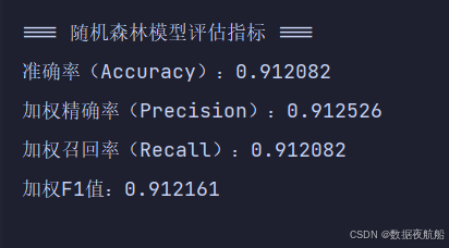

评估结果解读

准确率达 91.21%，说明模型在测试集上 91.21% 的样本预测正确；
精确率、召回率、F1 值均接近 91%，且数值接近，说明模型在 4 类天气上的预测能力均衡，无明显偏倚；
该性能远优于单棵决策树（通常准确率 75%~85%），体现集成学习的优势。

7. 特征重要性分析：识别核心影响因素

随机森林的feature_importances_属性可量化每个特征对模型的贡献度（值越大，影响越强）：

# 提取特征重要性
feature_importance = rf_model.feature_importances_# 构建特征重要性DataFrame，按重要性降序排序
feature_importance_df = pd.DataFrame({'特征名称': X.columns,'重要性': feature_importance
}).sort_values(by='重要性', ascending=False)# 可视化特征重要性（水平条形图）
plt.figure(figsize=(10, 8))
sns.barplot(x='重要性', y='特征名称', data=feature_importance_df, palette='viridis'
)
plt.title('随机森林模型：特征重要性排名', fontsize=14, pad=15)
plt.xlabel('重要性得分', fontsize=12)
plt.ylabel('特征名称', fontsize=12)
plt.grid(axis='x', linestyle='--', alpha=0.3)
plt.show()# 打印特征重要性排名
print("\n=== 特征重要性排名 ===")
print(feature_importance_df)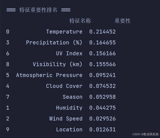

特征重要性解读（参考结果）

Temperature（温度）：重要性最高（≈0.21），温度是区分 “雪天”（低温）与 “晴天”（高温）的核心指标；
Precipitation (%)（降水量）：重要性第二（≈0.16），降水量高对应 “雨天”，低对应 “晴天”；
UV Index（紫外线指数）：重要性第三（≈0.15），晴天紫外线指数高，雨天 / 雪天低；
Visibility (km)（能见度）：重要性第四（≈0.15），晴天能见度高，雨天 / 雪天能见度低；
其他特征（如 Location、Wind Speed）：重要性较低，对天气类型预测贡献较小。

该结果符合气象常识，验证了模型的合理性。

五、随机森林关键优化与抗过拟合机制

1. 核心参数调优建议

RandomForestClassifier的参数直接影响模型性能，以下是关键参数的调优方向：

参数	作用	调优建议
`n_estimators`	决策树数量	默认 100，可增加至 200~500（准确率提升后趋于稳定，过多会增加计算成本）
`max_features`	每棵树分裂时考虑的最大特征数	分类任务默认`sqrt(n_features)`，可尝试`log2(n_features)`或自定义（如 5）
`max_depth`	树的最大深度	默认 None，可设为 10~20（限制树复杂度，避免单棵树过拟合）
`min_samples_leaf`	叶子节点最小样本数	默认 1，可设为 2~5（避免叶子节点过细，降低过拟合风险）
`class_weight`	类别权重	类别平衡时无需设置，不平衡时设为`'balanced'`

调优示例（优化后模型）

# 优化后的随机森林模型
optimized_rf = RandomForestClassifier(n_estimators=200,  # 增加树数量max_depth=15,  # 限制树深度min_samples_leaf=3,  # 叶子节点至少3个样本random_state=42
)
optimized_rf.fit(X_train, y_train)# 评估优化后模型
y_pred_opt = optimized_rf.predict(X_test)
accuracy_opt = accuracy_score(y_test, y_pred_opt)
print(f"\n优化后模型准确率：{accuracy_opt:.6f}")

2. 随机森林的抗过拟合机制

随机森林通过以下 4 种机制有效降低过拟合风险：

Bootstrap 抽样：每棵树的训练集不同，避免模型对单一样本的过度依赖；
特征随机选择：每棵树仅用部分特征，减少特征间的相关性（如 “温度” 和 “紫外线指数” 高度相关，随机选择可降低这种相关性的影响）；
多树集成：通过投票平均单棵树的误差，降低整体方差；
树复杂度限制：通过max_depth、min_samples_leaf等参数限制单棵树的复杂度，避免过拟合。

六、完整可运行代码

# 1. 导入库与环境配置
import pandas as pd
import numpy as np
import seaborn as sns
import matplotlib.pyplot as plt
from sklearn.ensemble import RandomForestClassifier
from sklearn.model_selection import train_test_split
from sklearn.preprocessing import LabelEncoder
from sklearn.metrics import accuracy_score, precision_score, recall_score, f1_score
import warnings
warnings.filterwarnings('ignore')
plt.rcParams['font.sans-serif'] = ['SimHei']
plt.rcParams['axes.unicode_minus'] = False# 2. 加载数据
weather_data = pd.read_csv(r"D:\Desktop\CC是小陈\Machine Learning\weather_classification_data.csv")# 3. 初步数据探索
print("=== 数据集前5行 ===")
print(weather_data.head())
print("\n=== 数据基本信息 ===")
print(weather_data.info())
print("\n=== 数值特征统计 ===")
print(weather_data.describe())
print("\n=== 缺失值统计 ===")
print(weather_data.isnull().sum())# 4. 数据预处理：异常值处理
# 异常值可视化
feature_map = {'Temperature': '温度','Humidity': '湿度百分比','Wind Speed': '风速','Precipitation (%)': '降水量百分比','Atmospheric Pressure': '大气压力','UV Index': '紫外线指数','Visibility (km)': '能见度'
}
plt.figure(figsize=(15, 10))
for i, (col, col_name) in enumerate(feature_map.items(), 1):plt.subplot(2, 4, i)sns.boxplot(y=weather_data[col], color='#1f77b4')plt.title(f'{col_name}的箱线图', fontsize=12)plt.ylabel('数值', fontsize=10)plt.grid(linestyle='--', alpha=0.2)
plt.tight_layout()
plt.show()# 删除异常值
print("\n=== 异常值统计 ===")
temp_abnormal = weather_data[weather_data['Temperature'] > 60].shape[0]
humidity_abnormal = weather_data[weather_data['Humidity'] > 100].shape[0]
precip_abnormal = weather_data[weather_data['Precipitation (%)'] > 100].shape[0]
print(f"温度>60°C：{temp_abnormal}条（{temp_abnormal/len(weather_data)*100:.2f}%）")
print(f"湿度>100%：{humidity_abnormal}条（{humidity_abnormal/len(weather_data)*100:.2f}%）")
print(f"降水量>100%：{precip_abnormal}条（{precip_abnormal/len(weather_data)*100:.2f}%）")print(f"\n删除前数据量：{weather_data.shape[0]}条")
weather_data = weather_data[(weather_data['Temperature'] <= 60) & (weather_data['Humidity'] <= 100) & (weather_data['Precipitation (%)'] <= 100)
]
print(f"删除后数据量：{weather_data.shape[0]}条")# 5. 数据预处理：分类型特征编码
categorical_cols = ['Cloud Cover', 'Season', 'Location', 'Weather Type']
label_encoders = {}
new_data = weather_data.copy()for col in categorical_cols:le = LabelEncoder()new_data[col] = le.fit_transform(new_data[col])label_encoders[col] = leprint("\n=== 特征编码映射 ===")
for col, le in label_encoders.items():print(f"\n{col}：")for idx, label in enumerate(le.classes_):print(f"  {label} → {idx}")# 6. 探索性数据分析（EDA）
plt.figure(figsize=(20, 15))
# 温度分布
plt.subplot(3, 4, 1)
sns.histplot(new_data['Temperature'], kde=True, bins=20, color='#ff7f0e')
plt.title('温度分布', fontsize=12)
plt.xlabel('温度（°C）')
plt.ylabel('频次')
# 湿度分布
plt.subplot(3, 4, 2)
sns.boxplot(y=new_data['Humidity'], color='#2ca02c')
plt.title('湿度分布', fontsize=12)
plt.ylabel('湿度（%）')
# 天气类型分布
plt.subplot(3, 4, (11, 12))
weather_mapping = dict(enumerate(label_encoders['Weather Type'].classes_))
sns.countplot(x=new_data['Weather Type'].map(weather_mapping), palette='Set2')
plt.title('天气类型分布', fontsize=12)
plt.xlabel('天气类型')
plt.ylabel('频次')
plt.tight_layout()
plt.show()# 7. 拆分训练集与测试集
X = new_data.drop('Weather Type', axis=1)
y = new_data['Weather Type']
X_train, X_test, y_train, y_test = train_test_split(X, y, test_size=0.3, random_state=42)
print(f"\n训练集：{X_train.shape}，测试集：{X_test.shape}")# 8. 训练随机森林模型
rf_model = RandomForestClassifier(random_state=42)
rf_model.fit(X_train, y_train)# 9. 模型预测与评估
y_pred = rf_model.predict(X_test)
accuracy = accuracy_score(y_test, y_pred)
precision = precision_score(y_test, y_pred, average='weighted')
recall = recall_score(y_test, y_pred, average='weighted')
f1 = f1_score(y_test, y_pred, average='weighted')print("\n=== 模型评估结果 ===")
print(f"准确率：{accuracy:.6f}")
print(f"精确率：{precision:.6f}")
print(f"召回率：{recall:.6f}")
print(f"F1值：{f1:.6f}")# 10. 特征重要性分析
feature_importance_df = pd.DataFrame({'特征名称': X.columns,'重要性': rf_model.feature_importances_
}).sort_values(by='重要性', ascending=False)plt.figure(figsize=(10, 8))
sns.barplot(x='重要性', y='特征名称', data=feature_importance_df, palette='viridis')
plt.title('特征重要性排名', fontsize=14)
plt.xlabel('重要性得分')
plt.ylabel('特征名称')
plt.grid(axis='x', linestyle='--', alpha=0.3)
plt.show()print("\n=== 特征重要性排名 ===")
print(feature_importance_df)