当前位置：首页 > news >正文

深度学习实战指南：从神经网络基础到模型优化的完整攻略

news 2025/9/15 5:20:55

在这里插入图片描述

🌟 Hello，我是蒋星熠Jaxonic！
🌈 在浩瀚无垠的技术宇宙中，我是一名执着的星际旅人，用代码绘制探索的轨迹。
🚀 每一个算法都是我点燃的推进器，每一行代码都是我航行的星图。
🔭 每一次性能优化都是我的天文望远镜，每一次架构设计都是我的引力弹弓。
🎻 在数字世界的协奏曲中，我既是作曲家也是首席乐手。让我们携手，在二进制星河中谱写属于极客的壮丽诗篇！

摘要

作为一名在AI领域深耕多年的技术探索者，我深深被深度学习的魅力所震撼。从最初接触感知机的那个午后，到如今能够构建复杂的神经网络架构，这段旅程充满了挑战与惊喜。深度学习不仅仅是一种技术，更是一种思维方式的革命——它让机器拥有了"学习"的能力，让数据变成了智慧的源泉。

在这个信息爆炸的时代，深度学习已经成为推动人工智能发展的核心引擎。从计算机视觉到自然语言处理，从推荐系统到自动驾驶，深度学习的应用无处不在。然而，对于许多初学者来说，深度学习仍然是一个充满神秘色彩的黑盒子。复杂的数学公式、繁多的网络架构、以及各种优化技巧，往往让人望而却步。

本文将以我多年的实战经验为基础，为大家构建一个从理论到实践的完整学习路径。我们将从神经网络的基本原理出发，逐步深入到卷积神经网络、循环神经网络等高级架构，并通过丰富的代码示例和可视化图表，让抽象的概念变得具体可感。同时，我还会分享在实际项目中遇到的各种挑战和解决方案，包括数据预处理、模型调优、过拟合防止等关键技术点。

无论你是刚刚踏入AI领域的新手，还是希望深化理解的进阶开发者，这篇文章都将为你提供有价值的指导。让我们一起踏上这段激动人心的深度学习之旅，用代码点亮智能的火花，用算法编织未来的蓝图！

1. 深度学习基础理论

1.1 神经网络的生物学启发

深度学习的核心思想源于对人脑神经元工作机制的模拟。每个人工神经元都是对生物神经元的简化抽象，通过接收多个输入信号，经过加权求和和激活函数处理后，产生输出信号。

import numpy as np
import matplotlib.pyplot as plt
from sklearn.datasets import make_classification
from sklearn.model_selection import train_test_splitclass Neuron:"""单个神经元的实现"""def __init__(self, input_size):# 初始化权重和偏置self.weights = np.random.randn(input_size) * 0.1self.bias = np.random.randn() * 0.1def sigmoid(self, x):"""Sigmoid激活函数"""return 1 / (1 + np.exp(-np.clip(x, -500, 500)))  # 防止溢出def forward(self, inputs):"""前向传播"""# 计算加权和weighted_sum = np.dot(inputs, self.weights) + self.bias# 应用激活函数output = self.sigmoid(weighted_sum)return output, weighted_sumdef backward(self, inputs, error):"""反向传播更新权重"""learning_rate = 0.1# 计算梯度gradient = error * inputs# 更新权重和偏置self.weights -= learning_rate * gradientself.bias -= learning_rate * error# 创建示例数据
X, y = make_classification(n_samples=1000, n_features=2, n_redundant=0, n_informative=2, n_clusters_per_class=1, random_state=42)
X_train, X_test, y_train, y_test = train_test_split(X, y, test_size=0.2, random_state=42)# 创建并训练单个神经元
neuron = Neuron(input_size=2)
print(f"初始权重: {neuron.weights}")
print(f"初始偏置: {neuron.bias}")

这段代码展示了单个神经元的基本结构，包括权重初始化、前向传播和反向传播的核心逻辑。

1.2 多层感知机架构

单个神经元的表达能力有限，通过堆叠多层神经元可以构建更强大的模型。多层感知机（MLP）是最基础的深度学习架构。

在这里插入图片描述

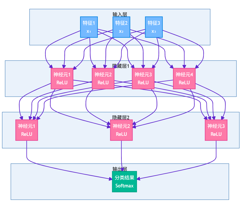
图1：多层感知机架构图 - 展示深度神经网络的层次结构

import torch
import torch.nn as nn
import torch.optim as optim
from torch.utils.data import DataLoader, TensorDatasetclass MLP(nn.Module):"""多层感知机实现"""def __init__(self, input_size, hidden_sizes, output_size, dropout_rate=0.2):super(MLP, self).__init__()layers = []prev_size = input_size# 构建隐藏层for hidden_size in hidden_sizes:layers.append(nn.Linear(prev_size, hidden_size))layers.append(nn.ReLU())layers.append(nn.Dropout(dropout_rate))  # 防止过拟合prev_size = hidden_size# 输出层layers.append(nn.Linear(prev_size, output_size))self.network = nn.Sequential(*layers)def forward(self, x):return self.network(x)# 模型配置
input_size = 784  # MNIST图像大小 28x28
hidden_sizes = [512, 256, 128]  # 三个隐藏层
output_size = 10  # 10个数字类别
dropout_rate = 0.3# 创建模型
model = MLP(input_size, hidden_sizes, output_size, dropout_rate)# 定义损失函数和优化器
criterion = nn.CrossEntropyLoss()
optimizer = optim.Adam(model.parameters(), lr=0.001, weight_decay=1e-4)print(f"模型参数总数: {sum(p.numel() for p in model.parameters())}")
print(f"模型结构:\n{model}")

这个MLP实现展示了如何构建深层网络，包括Dropout正则化和权重衰减等防止过拟合的技术。

2. 卷积神经网络（CNN）

2.1 卷积操作的数学原理

卷积神经网络通过卷积操作提取图像的局部特征，这种操作具有平移不变性和参数共享的优势。

import torch.nn.functional as Fdef visualize_convolution():"""可视化卷积操作"""# 创建示例输入图像 (1, 1, 5, 5)input_image = torch.tensor([[[[1, 2, 3, 0, 1],[4, 5, 6, 1, 2],[7, 8, 9, 2, 3],[1, 2, 3, 4, 5],[2, 3, 4, 5, 6]]]], dtype=torch.float32)# 定义卷积核 (边缘检测)edge_kernel = torch.tensor([[[[-1, -1, -1],[-1,  8, -1],[-1, -1, -1]]]], dtype=torch.float32)# 执行卷积操作output = F.conv2d(input_image, edge_kernel, padding=1)print("输入图像:")print(input_image.squeeze().numpy())print("\n卷积核 (边缘检测):")print(edge_kernel.squeeze().numpy())print("\n卷积结果:")print(output.squeeze().numpy())return input_image, edge_kernel, output# 执行可视化
input_img, kernel, conv_output = visualize_convolution()

2.2 完整的CNN架构实现

class CNN(nn.Module):"""卷积神经网络实现"""def __init__(self, num_classes=10):super(CNN, self).__init__()# 第一个卷积块self.conv1 = nn.Conv2d(1, 32, kernel_size=3, padding=1)self.bn1 = nn.BatchNorm2d(32)  # 批归一化self.pool1 = nn.MaxPool2d(2, 2)# 第二个卷积块self.conv2 = nn.Conv2d(32, 64, kernel_size=3, padding=1)self.bn2 = nn.BatchNorm2d(64)self.pool2 = nn.MaxPool2d(2, 2)# 第三个卷积块self.conv3 = nn.Conv2d(64, 128, kernel_size=3, padding=1)self.bn3 = nn.BatchNorm2d(128)self.pool3 = nn.MaxPool2d(2, 2)# 全连接层self.fc1 = nn.Linear(128 * 3 * 3, 512)self.dropout = nn.Dropout(0.5)self.fc2 = nn.Linear(512, num_classes)def forward(self, x):# 卷积块1x = self.pool1(F.relu(self.bn1(self.conv1(x))))# 卷积块2x = self.pool2(F.relu(self.bn2(self.conv2(x))))# 卷积块3x = self.pool3(F.relu(self.bn3(self.conv3(x))))# 展平x = x.view(x.size(0), -1)# 全连接层x = F.relu(self.fc1(x))x = self.dropout(x)x = self.fc2(x)return x# 创建CNN模型
cnn_model = CNN(num_classes=10)
print(f"CNN模型参数总数: {sum(p.numel() for p in cnn_model.parameters())}")

这个CNN实现包含了批归一化、Dropout等现代深度学习技术，能够有效处理图像分类任务。

在这里插入图片描述

图2：CNN前向传播时序图 - 展示数据在网络中的流动过程

3. 循环神经网络（RNN）与长短期记忆网络（LSTM）

3.1 RNN的序列建模能力

循环神经网络专门用于处理序列数据，通过隐藏状态在时间步之间传递信息。

class SimpleRNN(nn.Module):"""简单RNN实现"""def __init__(self, input_size, hidden_size, output_size, num_layers=1):super(SimpleRNN, self).__init__()self.hidden_size = hidden_sizeself.num_layers = num_layers# RNN层self.rnn = nn.RNN(input_size, hidden_size, num_layers, batch_first=True, dropout=0.2)# 输出层self.fc = nn.Linear(hidden_size, output_size)def forward(self, x):# 初始化隐藏状态h0 = torch.zeros(self.num_layers, x.size(0), self.hidden_size)# RNN前向传播out, _ = self.rnn(x, h0)# 取最后一个时间步的输出out = self.fc(out[:, -1, :])return out# 创建RNN模型用于文本分类
vocab_size = 10000
embedding_dim = 128
hidden_size = 256
num_classes = 5class TextClassifierRNN(nn.Module):"""基于RNN的文本分类器"""def __init__(self, vocab_size, embedding_dim, hidden_size, num_classes):super(TextClassifierRNN, self).__init__()# 词嵌入层self.embedding = nn.Embedding(vocab_size, embedding_dim)# LSTM层 (比RNN更强大)self.lstm = nn.LSTM(embedding_dim, hidden_size, batch_first=True, bidirectional=True)# 注意力机制self.attention = nn.Linear(hidden_size * 2, 1)# 分类层self.classifier = nn.Linear(hidden_size * 2, num_classes)self.dropout = nn.Dropout(0.3)def forward(self, x):# 词嵌入embedded = self.embedding(x)  # (batch_size, seq_len, embedding_dim)# LSTM处理lstm_out, _ = self.lstm(embedded)  # (batch_size, seq_len, hidden_size*2)# 注意力权重计算attention_weights = torch.softmax(self.attention(lstm_out), dim=1)# 加权平均context_vector = torch.sum(attention_weights * lstm_out, dim=1)# 分类output = self.classifier(self.dropout(context_vector))return output# 创建文本分类模型
text_model = TextClassifierRNN(vocab_size, embedding_dim, hidden_size, num_classes)
print(f"文本分类模型参数总数: {sum(p.numel() for p in text_model.parameters())}")

这个实现展示了如何使用LSTM和注意力机制构建强大的文本分类器。

3.2 训练过程可视化

在这里插入图片描述

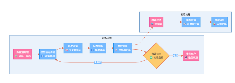
图3：深度学习训练流程图 - 展示完整的模型训练和验证过程

4. 模型优化与调参策略

4.1 学习率调度策略

学习率是深度学习中最重要的超参数之一，合适的学习率调度策略能显著提升模型性能。

import torch.optim.lr_scheduler as lr_scheduler
import matplotlib.pyplot as pltdef compare_lr_schedulers():"""比较不同学习率调度策略"""# 创建示例模型和优化器model = nn.Linear(10, 1)# 不同的调度器schedulers = {'StepLR': lr_scheduler.StepLR(optim.SGD(model.parameters(), lr=0.1), step_size=30, gamma=0.1),'ExponentialLR': lr_scheduler.ExponentialLR(optim.SGD(model.parameters(), lr=0.1), gamma=0.95),'CosineAnnealingLR': lr_scheduler.CosineAnnealingLR(optim.SGD(model.parameters(), lr=0.1), T_max=100),'ReduceLROnPlateau': lr_scheduler.ReduceLROnPlateau(optim.SGD(model.parameters(), lr=0.1), mode='min', factor=0.5, patience=10)}# 模拟训练过程epochs = 100lr_history = {name: [] for name in schedulers.keys()}for name, scheduler in schedulers.items():if name != 'ReduceLROnPlateau':for epoch in range(epochs):lr_history[name].append(scheduler.get_last_lr()[0])scheduler.step()else:# ReduceLROnPlateau需要损失值for epoch in range(epochs):lr_history[name].append(scheduler.optimizer.param_groups[0]['lr'])# 模拟损失下降然后平稳fake_loss = max(1.0 - epoch * 0.01, 0.1) + 0.05 * (epoch > 50)scheduler.step(fake_loss)return lr_history# 执行比较
lr_comparison = compare_lr_schedulers()
print("学习率调度策略比较完成")# 训练监控类
class TrainingMonitor:"""训练过程监控"""def __init__(self):self.train_losses = []self.val_losses = []self.train_accuracies = []self.val_accuracies = []self.learning_rates = []def update(self, train_loss, val_loss, train_acc, val_acc, lr):self.train_losses.append(train_loss)self.val_losses.append(val_loss)self.train_accuracies.append(train_acc)self.val_accuracies.append(val_acc)self.learning_rates.append(lr)def plot_metrics(self):"""绘制训练指标"""fig, axes = plt.subplots(2, 2, figsize=(12, 8))# 损失曲线axes[0, 0].plot(self.train_losses, label='训练损失', color='blue')axes[0, 0].plot(self.val_losses, label='验证损失', color='red')axes[0, 0].set_title('损失变化')axes[0, 0].legend()# 准确率曲线axes[0, 1].plot(self.train_accuracies, label='训练准确率', color='green')axes[0, 1].plot(self.val_accuracies, label='验证准确率', color='orange')axes[0, 1].set_title('准确率变化')axes[0, 1].legend()# 学习率变化axes[1, 0].plot(self.learning_rates, color='purple')axes[1, 0].set_title('学习率变化')plt.tight_layout()return figmonitor = TrainingMonitor()

4.2 正则化技术对比

正则化技术	原理	适用场景	优点	缺点
Dropout	随机丢弃神经元	全连接层	简单有效，防止过拟合	增加训练时间
Batch Normalization	批次归一化	卷积层、全连接层	加速收敛，稳定训练	依赖批次大小
L1/L2正则化	权重惩罚	所有层	数学理论完善	需要调节正则化系数
Early Stopping	提前停止训练	训练过程	防止过拟合，节省时间	需要验证集
Data Augmentation	数据增强	图像、文本	增加数据多样性	可能引入噪声

class RegularizedModel(nn.Module):"""集成多种正则化技术的模型"""def __init__(self, input_size, hidden_sizes, output_size, dropout_rate=0.3, use_batch_norm=True):super(RegularizedModel, self).__init__()self.layers = nn.ModuleList()self.batch_norms = nn.ModuleList()self.use_batch_norm = use_batch_normprev_size = input_sizefor hidden_size in hidden_sizes:# 线性层self.layers.append(nn.Linear(prev_size, hidden_size))# 批归一化if use_batch_norm:self.batch_norms.append(nn.BatchNorm1d(hidden_size))prev_size = hidden_size# 输出层self.output_layer = nn.Linear(prev_size, output_size)self.dropout = nn.Dropout(dropout_rate)def forward(self, x):for i, layer in enumerate(self.layers):x = layer(x)# 批归一化if self.use_batch_norm:x = self.batch_norms[i](x)# 激活函数x = F.relu(x)# Dropoutx = self.dropout(x)# 输出层x = self.output_layer(x)return x# 创建正则化模型
regularized_model = RegularizedModel(input_size=784, hidden_sizes=[512, 256, 128], output_size=10,dropout_rate=0.3,use_batch_norm=True
)

5. 深度学习框架对比与选择

5.1 主流框架特点分析

在这里插入图片描述

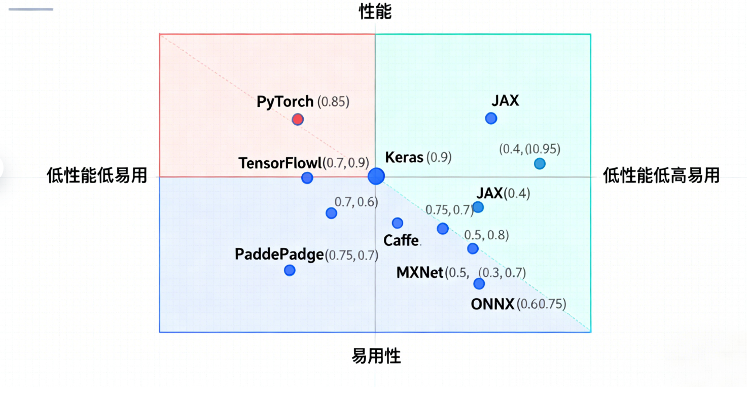
图4：深度学习框架对比象限图 - 展示各框架在性能和易用性方面的定位

5.2 模型部署策略

import torch.jit
import onnx
import onnxruntimeclass ModelDeployment:"""模型部署工具类"""@staticmethoddef export_to_torchscript(model, example_input, save_path):"""导出为TorchScript格式"""model.eval()# 追踪模式traced_model = torch.jit.trace(model, example_input)traced_model.save(save_path)print(f"模型已导出为TorchScript: {save_path}")return traced_model@staticmethoddef export_to_onnx(model, example_input, save_path):"""导出为ONNX格式"""model.eval()torch.onnx.export(model,example_input,save_path,export_params=True,opset_version=11,do_constant_folding=True,input_names=['input'],output_names=['output'],dynamic_axes={'input': {0: 'batch_size'},'output': {0: 'batch_size'}})print(f"模型已导出为ONNX: {save_path}")@staticmethoddef benchmark_inference(model, test_data, num_runs=100):"""推理性能基准测试"""import timemodel.eval()times = []with torch.no_grad():# 预热for _ in range(10):_ = model(test_data)# 正式测试for _ in range(num_runs):start_time = time.time()_ = model(test_data)end_time = time.time()times.append(end_time - start_time)avg_time = sum(times) / len(times)print(f"平均推理时间: {avg_time*1000:.2f}ms")print(f"吞吐量: {1/avg_time:.2f} samples/sec")return avg_time# 使用示例
deployment = ModelDeployment()# 创建示例模型和数据
example_model = CNN(num_classes=10)
example_input = torch.randn(1, 1, 28, 28)# 导出模型
# deployment.export_to_torchscript(example_model, example_input, "model.pt")
# deployment.export_to_onnx(example_model, example_input, "model.onnx")

6. 实战项目：图像分类完整流程

6.1 数据预处理管道

from torchvision import transforms, datasets
from torch.utils.data import DataLoader
import albumentations as A
from albumentations.pytorch import ToTensorV2class DataPipeline:"""数据处理管道"""def __init__(self, data_dir, batch_size=32, image_size=224):self.data_dir = data_dirself.batch_size = batch_sizeself.image_size = image_size# 训练时的数据增强self.train_transform = A.Compose([A.Resize(image_size, image_size),A.HorizontalFlip(p=0.5),A.RandomBrightnessContrast(p=0.3),A.ShiftScaleRotate(shift_limit=0.1, scale_limit=0.1, rotate_limit=15, p=0.3),A.CoarseDropout(max_holes=8, max_height=32, max_width=32, p=0.3),A.Normalize(mean=[0.485, 0.456, 0.406], std=[0.229, 0.224, 0.225]),ToTensorV2()])# 验证时的变换self.val_transform = A.Compose([A.Resize(image_size, image_size),A.Normalize(mean=[0.485, 0.456, 0.406], std=[0.229, 0.224, 0.225]),ToTensorV2()])def get_dataloaders(self):"""获取数据加载器"""# 这里使用CIFAR-10作为示例train_dataset = datasets.CIFAR10(root=self.data_dir, train=True, download=True,transform=transforms.Compose([transforms.ToPILImage(),transforms.Lambda(lambda x: self.train_transform(image=np.array(x))['image'])]))val_dataset = datasets.CIFAR10(root=self.data_dir, train=False, download=True,transform=transforms.Compose([transforms.ToPILImage(),transforms.Lambda(lambda x: self.val_transform(image=np.array(x))['image'])]))train_loader = DataLoader(train_dataset, batch_size=self.batch_size, shuffle=True, num_workers=4, pin_memory=True)val_loader = DataLoader(val_dataset, batch_size=self.batch_size, shuffle=False, num_workers=4, pin_memory=True)return train_loader, val_loader# 创建数据管道
data_pipeline = DataPipeline('./data', batch_size=64, image_size=32)

6.2 完整训练循环

from tqdm import tqdm
import wandb  # 实验跟踪工具class Trainer:"""训练器类"""def __init__(self, model, train_loader, val_loader, criterion, optimizer, scheduler=None, device='cuda'):self.model = model.to(device)self.train_loader = train_loaderself.val_loader = val_loaderself.criterion = criterionself.optimizer = optimizerself.scheduler = schedulerself.device = deviceself.monitor = TrainingMonitor()def train_epoch(self):"""训练一个epoch"""self.model.train()total_loss = 0correct = 0total = 0pbar = tqdm(self.train_loader, desc='Training')for batch_idx, (data, target) in enumerate(pbar):data, target = data.to(self.device), target.to(self.device)# 前向传播self.optimizer.zero_grad()output = self.model(data)loss = self.criterion(output, target)# 反向传播loss.backward()# 梯度裁剪torch.nn.utils.clip_grad_norm_(self.model.parameters(), max_norm=1.0)self.optimizer.step()# 统计total_loss += loss.item()pred = output.argmax(dim=1, keepdim=True)correct += pred.eq(target.view_as(pred)).sum().item()total += target.size(0)# 更新进度条pbar.set_postfix({'Loss': f'{loss.item():.4f}','Acc': f'{100.*correct/total:.2f}%'})avg_loss = total_loss / len(self.train_loader)accuracy = 100. * correct / totalreturn avg_loss, accuracydef validate(self):"""验证模型"""self.model.eval()total_loss = 0correct = 0total = 0with torch.no_grad():for data, target in tqdm(self.val_loader, desc='Validation'):data, target = data.to(self.device), target.to(self.device)output = self.model(data)loss = self.criterion(output, target)total_loss += loss.item()pred = output.argmax(dim=1, keepdim=True)correct += pred.eq(target.view_as(pred)).sum().item()total += target.size(0)avg_loss = total_loss / len(self.val_loader)accuracy = 100. * correct / totalreturn avg_loss, accuracydef train(self, epochs):"""完整训练流程"""best_val_acc = 0for epoch in range(epochs):print(f'\nEpoch {epoch+1}/{epochs}')# 训练train_loss, train_acc = self.train_epoch()# 验证val_loss, val_acc = self.validate()# 学习率调度if self.scheduler:if isinstance(self.scheduler, lr_scheduler.ReduceLROnPlateau):self.scheduler.step(val_loss)else:self.scheduler.step()# 记录指标current_lr = self.optimizer.param_groups[0]['lr']self.monitor.update(train_loss, val_loss, train_acc, val_acc, current_lr)# 保存最佳模型if val_acc > best_val_acc:best_val_acc = val_acctorch.save({'epoch': epoch,'model_state_dict': self.model.state_dict(),'optimizer_state_dict': self.optimizer.state_dict(),'val_acc': val_acc,}, 'best_model.pth')print(f'Train Loss: {train_loss:.4f}, Train Acc: {train_acc:.2f}%')print(f'Val Loss: {val_loss:.4f}, Val Acc: {val_acc:.2f}%')print(f'Learning Rate: {current_lr:.6f}')# 创建训练器并开始训练
model = CNN(num_classes=10)
criterion = nn.CrossEntropyLoss()
optimizer = optim.AdamW(model.parameters(), lr=0.001, weight_decay=1e-4)
scheduler = lr_scheduler.CosineAnnealingLR(optimizer, T_max=100)# trainer = Trainer(model, train_loader, val_loader, criterion, optimizer, scheduler)
# trainer.train(epochs=50)

7. 性能优化与加速技术

7.1 混合精度训练

from torch.cuda.amp import GradScaler, autocastclass MixedPrecisionTrainer(Trainer):"""混合精度训练器"""def __init__(self, *args, **kwargs):super().__init__(*args, **kwargs)self.scaler = GradScaler()def train_epoch(self):"""使用混合精度的训练epoch"""self.model.train()total_loss = 0correct = 0total = 0pbar = tqdm(self.train_loader, desc='Mixed Precision Training')for batch_idx, (data, target) in enumerate(pbar):data, target = data.to(self.device), target.to(self.device)self.optimizer.zero_grad()# 使用autocast进行前向传播with autocast():output = self.model(data)loss = self.criterion(output, target)# 缩放损失并反向传播self.scaler.scale(loss).backward()# 梯度裁剪self.scaler.unscale_(self.optimizer)torch.nn.utils.clip_grad_norm_(self.model.parameters(), max_norm=1.0)# 更新参数self.scaler.step(self.optimizer)self.scaler.update()# 统计total_loss += loss.item()pred = output.argmax(dim=1, keepdim=True)correct += pred.eq(target.view_as(pred)).sum().item()total += target.size(0)pbar.set_postfix({'Loss': f'{loss.item():.4f}','Acc': f'{100.*correct/total:.2f}%'})avg_loss = total_loss / len(self.train_loader)accuracy = 100. * correct / totalreturn avg_loss, accuracy

7.2 模型压缩技术

import torch.nn.utils.prune as pruneclass ModelCompression:"""模型压缩工具"""@staticmethoddef structured_pruning(model, pruning_ratio=0.3):"""结构化剪枝"""for name, module in model.named_modules():if isinstance(module, nn.Conv2d) or isinstance(module, nn.Linear):prune.ln_structured(module, name='weight', amount=pruning_ratio, n=2, dim=0)return model@staticmethoddef unstructured_pruning(model, pruning_ratio=0.3):"""非结构化剪枝"""parameters_to_prune = []for name, module in model.named_modules():if isinstance(module, nn.Conv2d) or isinstance(module, nn.Linear):parameters_to_prune.append((module, 'weight'))prune.global_unstructured(parameters_to_prune,pruning_method=prune.L1Unstructured,amount=pruning_ratio,)return model@staticmethoddef quantization(model, calibration_loader):"""模型量化"""model.eval()# 准备量化model.qconfig = torch.quantization.get_default_qconfig('fbgemm')torch.quantization.prepare(model, inplace=True)# 校准with torch.no_grad():for data, _ in calibration_loader:model(data)# 转换为量化模型quantized_model = torch.quantization.convert(model, inplace=False)return quantized_model# 使用示例
compression = ModelCompression()
# pruned_model = compression.structured_pruning(model, pruning_ratio=0.3)

深度学习优化箴言

“在深度学习的世界里，数据是燃料，算法是引擎，而优化是驾驶技术。只有三者完美结合，才能在AI的赛道上驰骋千里。记住，模型的复杂度不是目标，解决问题的能力才是王道。”

8. 前沿技术与发展趋势

8.1 Transformer架构革命

import mathclass MultiHeadAttention(nn.Module):"""多头注意力机制"""def __init__(self, d_model, num_heads, dropout=0.1):super().__init__()assert d_model % num_heads == 0self.d_model = d_modelself.num_heads = num_headsself.d_k = d_model // num_headsself.w_q = nn.Linear(d_model, d_model)self.w_k = nn.Linear(d_model, d_model)self.w_v = nn.Linear(d_model, d_model)self.w_o = nn.Linear(d_model, d_model)self.dropout = nn.Dropout(dropout)def scaled_dot_product_attention(self, Q, K, V, mask=None):"""缩放点积注意力"""scores = torch.matmul(Q, K.transpose(-2, -1)) / math.sqrt(self.d_k)if mask is not None:scores = scores.masked_fill(mask == 0, -1e9)attention_weights = F.softmax(scores, dim=-1)attention_weights = self.dropout(attention_weights)output = torch.matmul(attention_weights, V)return output, attention_weightsdef forward(self, query, key, value, mask=None):batch_size = query.size(0)# 线性变换并重塑为多头Q = self.w_q(query).view(batch_size, -1, self.num_heads, self.d_k).transpose(1, 2)K = self.w_k(key).view(batch_size, -1, self.num_heads, self.d_k).transpose(1, 2)V = self.w_v(value).view(batch_size, -1, self.num_heads, self.d_k).transpose(1, 2)# 应用注意力attention_output, attention_weights = self.scaled_dot_product_attention(Q, K, V, mask)# 合并多头attention_output = attention_output.transpose(1, 2).contiguous().view(batch_size, -1, self.d_model)# 最终线性变换output = self.w_o(attention_output)return output, attention_weightsclass TransformerBlock(nn.Module):"""Transformer块"""def __init__(self, d_model, num_heads, d_ff, dropout=0.1):super().__init__()self.attention = MultiHeadAttention(d_model, num_heads, dropout)self.norm1 = nn.LayerNorm(d_model)self.norm2 = nn.LayerNorm(d_model)self.feed_forward = nn.Sequential(nn.Linear(d_model, d_ff),nn.ReLU(),nn.Dropout(dropout),nn.Linear(d_ff, d_model))self.dropout = nn.Dropout(dropout)def forward(self, x, mask=None):# 多头注意力 + 残差连接attn_output, _ = self.attention(x, x, x, mask)x = self.norm1(x + self.dropout(attn_output))# 前馈网络 + 残差连接ff_output = self.feed_forward(x)x = self.norm2(x + self.dropout(ff_output))return x# 创建Transformer模型
transformer_block = TransformerBlock(d_model=512, num_heads=8, d_ff=2048)
print(f"Transformer块参数数量: {sum(p.numel() for p in transformer_block.parameters())}")

8.2 性能对比分析

在这里插入图片描述

图5：深度学习模型性能趋势图 - 展示不同架构在标准任务上的表现

总结

回望这段深度学习的探索之旅，我深深感受到了技术演进的磅礴力量。从最初的感知机到如今的大型语言模型，每一次架构创新都在推动着人工智能的边界不断扩展。作为一名技术实践者，我见证了深度学习从学术象牙塔走向产业应用的全过程，也亲身体验了这项技术给各行各业带来的深刻变革。

在这篇文章中，我们系统地梳理了深度学习的核心概念和关键技术。从神经网络的基础原理出发，我们深入探讨了卷积神经网络在计算机视觉领域的突破性应用，分析了循环神经网络在序列建模方面的独特优势，并展望了Transformer架构带来的技术革命。通过丰富的代码示例和可视化图表，我们将抽象的数学概念转化为具体的工程实践，让每一个技术细节都变得触手可及。

特别值得强调的是，深度学习不仅仅是一种技术工具，更是一种全新的问题解决思维。它教会我们如何从数据中发现模式，如何构建端到端的学习系统，如何在复杂的优化空间中寻找最优解。这种思维方式的转变，对于我们理解和应对未来的技术挑战具有深远的意义。

在实际项目中，我深刻体会到了理论与实践之间的差距。书本上的算法需要经过无数次的调试和优化才能在真实场景中发挥作用。数据预处理的细节、模型架构的选择、超参数的调优、正则化技术的应用，每一个环节都可能成为项目成功的关键因素。这也是为什么我在文章中特别强调了工程实践的重要性，并提供了完整的代码实现和最佳实践指南。

展望未来，深度学习领域仍然充满了无限可能。自监督学习、多模态融合、神经架构搜索、联邦学习等新兴技术正在不断涌现。同时，模型的可解释性、公平性、安全性等问题也日益受到关注。作为技术从业者，我们需要保持持续学习的心态，既要掌握扎实的基础理论，也要紧跟技术发展的前沿动态。

最后，我想说的是，深度学习的魅力不仅在于其强大的技术能力，更在于它为我们打开了一扇通往智能未来的大门。在这个充满变革的时代，让我们携手前行，用代码编织梦想，用算法点亮未来，在人工智能的星辰大海中留下属于我们这一代技术人的足迹！

■ 我是蒋星熠Jaxonic！如果这篇文章在你的技术成长路上留下了印记
■ 👁 【关注】与我一起探索技术的无限可能，见证每一次突破
■ 👍 【点赞】为优质技术内容点亮明灯，传递知识的力量
■ 🔖 【收藏】将精华内容珍藏，随时回顾技术要点
■ 💬 【评论】分享你的独特见解，让思维碰撞出智慧火花
■ 🗳 【投票】用你的选择为技术社区贡献一份力量
■ 技术路漫漫，让我们携手前行，在代码的世界里摘取属于程序员的那片星辰大海！

参考链接

Deep Learning - Ian Goodfellow, Yoshua Bengio, Aaron Courville
PyTorch官方文档 - 深度学习框架完整指南
Papers With Code - 深度学习最新论文和代码实现
Distill.pub - 深度学习可视化解释
CS231n: Convolutional Neural Networks for Visual Recognition

关键词标签

#深度学习 #神经网络 #PyTorch #卷积神经网络 #Transformer

数学公式补充：

反向传播核心公式： $∂L∂w=∂L∂a⋅∂a∂z⋅∂z∂w\frac{\partial L}{\partial w} = \frac{\partial L}{\partial a} \cdot \frac{\partial a}{\partial z} \cdot \frac{\partial z}{\partial w}$