Boost电路:稳态和小信号分析
稳态分析
参考张卫平的《开关变换器的建模与控制》的1.3章节内容;伏秒平衡:在稳态下,一个开关周期内电感电流的增量是0,即
dIL(t)dt=0\frac{dI_{L}(t)}{dt} = 0dtdIL(t)=0。电荷平衡:在稳态下,一个开关周期内电容电压的增量是0,即
dVC(t)dt=0\frac{dV_{C}(t)}{dt} = 0dtdVC(t)=0。Vg(t)=VgV_{g}\left. (t \right.) = V_{g}Vg(t)=Vg+v^g(t){\widehat{v}}_{g}\left. (t \right.)vg(t),IL(t)=IL+i^L(t)I_{L}\left. (t \right.) = I_{L} + {\widehat{i}}_{L}\left. (t \right.)IL(t)=IL+iL(t),VC(t)=VC+v^c(t)V_{C}\left. (t \right.) = V_{C} + {\widehat{v}}_{c}\left. (t \right.)VC(t)=VC+vc(t),V(t)=V+v^(t)V\left. (t \right.) = V + \widehat{v}\left. (t \right.)V(t)=V+v(t),Iload(t)=Iload+i^load(t)I_{load}\left. (t \right.) = I_{load} + {\widehat{i}}_{load}\left. (t \right.)Iload(t)=Iload+iload(t),
D(t)=D+d^(t)D\left. (t \right.) = D + \widehat{d}\left. (t \right.)D(t)=D+d(t)。上式中前者表示直流量,后者表示扰动。
在稳态下,应该用直流量 X,U,Y \ \mathbf{X,U,Y\ } X,U,Y 来代替 x(t),u(t),y(t) \ \mathbf{x}(\mathbf{t}),\mathbf{u(t),y(t)\ } x(t),u(t),y(t) 来代替状态变量,然后得到新的稳态下的状态空间方程,如下所示:
[00]=A X+B UY=CX+EU{\begin{bmatrix}
0 \\
0
\end{bmatrix} = \mathbf{A\ X + B\ U}
}\mathbf{Y = CX + EU}[00]=A X+B UY=CX+EU
[00]=A X+B U[00]=[−RL1−DRon−(1−D)RC1L1−(1−D)L1(1−D)C10][ILVC]+[1L1RC1L1(1−D)−(1−D)L10−1C10][VgIloadVf]{\begin{bmatrix} 0 \\ 0 \end{bmatrix} = \mathbf{A\ X + B\ U} }{\begin{bmatrix} 0 \\ 0 \end{bmatrix} = \begin{bmatrix} \frac{- R_{L1} - DR_{on} - (1 - D)R_{C1}}{L_{1}} & \frac{- (1 - D)}{L_{1}} \\ \frac{(1 - D)}{C_{1}} & 0 \end{bmatrix}\begin{bmatrix} I_{L} \\ V_{C} \end{bmatrix} + \begin{bmatrix} \frac{1}{L_{1}} & \frac{R_{C1}}{L_{1}}(1 - D) & \frac{- (1 - D)}{L_{1}} \\ 0 & \frac{- 1}{C_{1}} & 0 \end{bmatrix}\begin{bmatrix} V_{g} \\ I_{load} \\ V_{f} \end{bmatrix}}[00]=A X+B U[00]=[L1−RL1−DRon−(1−D)RC1C1(1−D)L1−(1−D)0][ILVC]+[L110L1RC1(1−D)C1−1L1−(1−D)0]VgIloadVf
将其拆分为两项,分别是:
0=−RL1−DRon−(1−D)RC1L1IL−(1−D)L1VC+1L1Vg+RC1(1−D)L1Iload−(1−D)L1Vf0=(1−D)C1IL−1C1Iload{0 = \frac{- R_{L1} - DR_{on} - (1 - D)R_{C1}}{L_{1}}I_{L} - \frac{(1 - D)}{L_{1}}V_{C} + \frac{1}{L_{1}}V_{g} + \frac{R_{C1}(1 - D)}{L_{1}}I_{load} - \frac{(1 - D)}{L_{1}}V_{f}
}{0 = \frac{(1 - D)}{C_{1}}I_{L} - \frac{1}{C_{1}}I_{load}}0=L1−RL1−DRon−(1−D)RC1IL−L1(1−D)VC+L11Vg+L1RC1(1−D)Iload−L1(1−D)Vf0=C1(1−D)IL−C11Iload
后一项者可得
IL=Iload(1−D)I_{L} = \frac{I_{load}}{(1 - D)}IL=(1−D)Iload
代入前一项可得
0=−RL1−DRon−(1−D)RC1L1(1−D)Iload−(1−D)L1VC+1L1Vg+RC1L1(1−D) Iload−(1−D)L1Vf(1−D)L1VC=−RL1−DRon−(1−D)RC1L1(1−D)Iload−(1−D)L1VC+1L1Vg+RC1L1(1−D) Iload−(1−D)L1Vf{0 = \frac{- R_{L1} - DR_{on} - (1 - D)R_{C1}}{L_{1}(1 - D)}I_{load} - \frac{(1 - D)}{L_{1}}V_{C} + \frac{1}{L_{1}}V_{g} + \frac{R_{C1}}{L_{1}}(1 - D)\ I_{load} - \frac{(1 - D)}{L_{1}}V_{f}
}{\frac{(1 - D)}{L_{1}}V_{C} = \frac{- R_{L1} - DR_{on} - (1 - D)R_{C1}}{L_{1}(1 - D)}I_{load} - \frac{(1 - D)}{L_{1}}V_{C} + \frac{1}{L_{1}}V_{g} + \frac{R_{C1}}{L_{1}}(1 - D)\ I_{load} - \frac{(1 - D)}{L_{1}}V_{f}}0=L1(1−D)−RL1−DRon−(1−D)RC1Iload−L1(1−D)VC+L11Vg+L1RC1(1−D) Iload−L1(1−D)VfL1(1−D)VC=L1(1−D)−RL1−DRon−(1−D)RC1Iload−L1(1−D)VC+L11Vg+L1RC1(1−D) Iload−L1(1−D)Vf
可得
VC=−RL1−DRon−(1−D)RC1(1−D)2Iload+Vg(1−D)+RC1Iload−VfV_{C} = \frac{- R_{L1} - DR_{on} - (1 - D)R_{C1}}{{(1 - D)}^{2}}I_{load} + \frac{V_{g}}{(1 - D)} + R_{C1}I_{load} - V_{f}VC=(1−D)2−RL1−DRon−(1−D)RC1Iload+(1−D)Vg+RC1Iload−Vf
输出方程的稳态表达式如下
[V]=[(1−D)RC11][ILVC]+[0−RC10][VgIloadVf]\lbrack V\rbrack = \left\lbrack (1 - D)\begin{matrix}
R_{C1} & 1
\end{matrix} \right\rbrack\begin{bmatrix}
I_{L} \\
V_{C}
\end{bmatrix} + \begin{bmatrix}
0 & - R_{C1} & 0
\end{bmatrix}\begin{bmatrix}
V_{g} \\
I_{load} \\
V_{f}
\end{bmatrix}[V]=[(1−D)RC11][ILVC]+[0−RC10]VgIloadVf
可得
V=(1−D)RC1IL+VC−RC1Iload =(1−D)RC1Iload(1−D)+−RL1−DRon−(1−D)RC1(1−D)2Iload+Vg(1−D)+RC1Iload−Vf−RC1Iload=RC1Iload+−RL1−DRon−(1−D)RC1(1−D)2Iload+Vg(1−D)+RC1Iload−Vf−RC1Iload=RC1Iload−RC1(1−D)Iload−RL1+DRon(1−D)2Iload+Vg(1−D)−Vf=Vg(1−D)−Vf−D(1−D)RC1Iload−1(1−D)2RL1Iload−D(1−D)2RonIload{V = (1 - D)R_{C1}I_{L} + V_{C} - R_{C1}I_{load}
}{\ = (1 - D)R_{C1}\frac{I_{load}}{(1 - D)} + \frac{- R_{L1} - DR_{on} - (1 - D)R_{C1}}{(1 - D)^{2}}I_{load} + \frac{V_{g}}{(1 - D)} + R_{C1}I_{load} - V_{f} - R_{C1}I_{load}
}{= R_{C1}I_{load} + \frac{- R_{L1} - DR_{on} - (1 - D)R_{C1}}{(1 - D)^{2}}I_{load} + \frac{V_{g}}{(1 - D)} + R_{C1}I_{load} - V_{f} - R_{C1}I_{load}
}{= R_{C1}I_{load} - \frac{R_{C1}}{(1 - D)}I_{load} - \frac{R_{L1} + DR_{on}}{(1 - D)^{2}}I_{load} + \frac{V_{g}}{(1 - D)} - V_{f}
}{= \frac{V_{g}}{(1 - D)} - V_{f} - \frac{D}{(1 - D)}R_{C1}I_{load} - \frac{1}{(1 - D)^{2}}R_{L1}I_{load} - \frac{D}{(1 - D)^{2}}R_{on}I_{load}}V=(1−D)RC1IL+VC−RC1Iload =(1−D)RC1(1−D)Iload+(1−D)2−RL1−DRon−(1−D)RC1Iload+(1−D)Vg+RC1Iload−Vf−RC1Iload=RC1Iload+(1−D)2−RL1−DRon−(1−D)RC1Iload+(1−D)Vg+RC1Iload−Vf−RC1Iload=RC1Iload−(1−D)RC1Iload−(1−D)2RL1+DRonIload+(1−D)Vg−Vf=(1−D)Vg−Vf−(1−D)DRC1Iload−(1−D)21RL1Iload−(1−D)2DRonIload
由上式可知,由于VfV_{f}Vf,RC1R_{C1}RC1,RL1R_{L1}RL1,RonR_{on}Ron的存在,使得输出电压稳态值是和输出电流IloadI_{load}Iload相关联的。换言之,不同的输出电流,会让D发生调整,也会影响后续的各类小信号传递函数。
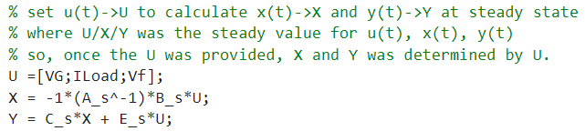
也可以用矩阵的形式直接计算,如下所示:
X=−A−1B UY=CX+EU=(E−CA−1B) U{\mathbf{X =} - \mathbf{A}^{\mathbf{- 1}}\mathbf{B\ U}
}{\mathbf{Y = CX + EU =}\left( \mathbf{E} - \mathbf{C}\mathbf{A}^{\mathbf{- 1}}\mathbf{B} \right)\mathbf{\ U}}X=−A−1B UY=CX+EU=(E−CA−1B) U
对应的MATLAB脚本如下
小信号模型分析
参考张卫平的《开关变换器的建模与控制》的1.3章节内容;完成稳态下的状态空间方程后,可以继续推导小信号模型,此时不仅用扰动量 x^(t), u^(t),y^(t) \ \widehat{\mathbf{x}}\mathbf{(t),\ }\widehat{\mathbf{u}}\mathbf{(t),}\widehat{\mathbf{y}}\mathbf{(t)\ } x(t), u(t),y(t) 来代替 x(t),u(t),y(t) \ \mathbf{x}(\mathbf{t}),\mathbf{u(t),y(t)\ } x(t),u(t),y(t) 来代替状态变量,具体如下:
dx^(t)dt=A x^(t)+B u^(t)+{(A1−A2)X−(B1−B2)U}d^(t)y^(t)=Cx^(t)+Eu^(t)+{(C1−C2)X−(E1−E2)U}d^(t){\frac{d\widehat{\mathbf{x}}\mathbf{(t)}}{dt} = \mathbf{A\ }\widehat{\mathbf{x}}\mathbf{(t) + B\ }\widehat{\mathbf{u}}\mathbf{(t) +}\left\{ \left( \mathbf{A}_{\mathbf{1}}\mathbf{-}\mathbf{A}_{\mathbf{2}} \right)\mathbf{X}\mathbf{-}\left( \mathbf{B}_{\mathbf{1}}\mathbf{-}\mathbf{B}_{\mathbf{2}} \right)\mathbf{U} \right\}\widehat{\mathbf{d}}\mathbf{(t)}
}{\widehat{\mathbf{y}}\mathbf{(t) = C}\widehat{\mathbf{x}}\mathbf{(t) + E}\widehat{\mathbf{u}}\mathbf{(t) +}\left\{ \left( \mathbf{C}_{\mathbf{1}}\mathbf{-}\mathbf{C}_{\mathbf{2}} \right)\mathbf{X}\mathbf{-}\left( \mathbf{E}_{\mathbf{1}}\mathbf{-}\mathbf{E}_{\mathbf{2}} \right)\mathbf{U} \right\}\widehat{\mathbf{d}}\mathbf{(t)}}dtdx(t)=A x(t)+B u(t)+{(A1−A2)X−(B1−B2)U}d(t)y(t)=Cx(t)+Eu(t)+{(C1−C2)X−(E1−E2)U}d(t)
其中,u^(t)\widehat{\mathbf{u}}(\mathbf{t})u(t)扰动信号,y^(t)\widehat{\mathbf{y}}(\mathbf{t})y(t)是输出信号,d^(t)\widehat{\mathbf{d}}\mathbf{(t)}d(t)是控制信号。接下来对上式进行拉普拉斯变换,可得( I\ \mathbf{I} I为单位矩阵):
sIx^(t)=A x^(s)+B u^(s)+[(A1−A2)X−(B1−B2)U]d^(s)y^(s)=Cx^(s)+Eu^(s)+[(C1−C2)X−(E1−E2)U]d^(s){\mathbf{sI}\widehat{\mathbf{x}}\mathbf{(t)} = \mathbf{A\ }\widehat{\mathbf{x}}\mathbf{(s) + B\ }\widehat{\mathbf{u}}\mathbf{(s) +}\left\lbrack \left( \mathbf{A}_{\mathbf{1}}\mathbf{-}\mathbf{A}_{\mathbf{2}} \right)\mathbf{X}\mathbf{-}\left( \mathbf{B}_{\mathbf{1}}\mathbf{-}\mathbf{B}_{\mathbf{2}} \right)\mathbf{U} \right\rbrack\widehat{\mathbf{d}}\mathbf{(s)}
}{\widehat{\mathbf{y}}\mathbf{(s) = C}\widehat{\mathbf{x}}\mathbf{(s) + E}\widehat{\mathbf{u}}\mathbf{(s) +}\left\lbrack \left( \mathbf{C}_{\mathbf{1}}\mathbf{-}\mathbf{C}_{\mathbf{2}} \right)\mathbf{X}\mathbf{-}\left( \mathbf{E}_{\mathbf{1}}\mathbf{-}\mathbf{E}_{\mathbf{2}} \right)\mathbf{U} \right\rbrack\widehat{\mathbf{d}}\mathbf{(s)}}sIx(t)=A x(s)+B u(s)+[(A1−A2)X−(B1−B2)U]d(s)y(s)=Cx(s)+Eu(s)+[(C1−C2)X−(E1−E2)U]d(s)
解得(下面会继续化简):
x^(t)=(sI−A)−1 B u^(s)+(sI−A)−1[(A1−A2)X−(B1−B2)U]d^(s)\widehat{\mathbf{x}}\mathbf{(t)} = \left( \mathbf{s}\mathbf{I} - \mathbf{A} \right)^{\mathbf{- 1}}\mathbf{\ B\ }\widehat{\mathbf{u}}\mathbf{(s) +}\left( \mathbf{s}\mathbf{I} - \mathbf{A} \right)^{\mathbf{- 1}}\left\lbrack \left( \mathbf{A}_{\mathbf{1}}\mathbf{-}\mathbf{A}_{\mathbf{2}} \right)\mathbf{X}\mathbf{-}\left( \mathbf{B}_{\mathbf{1}}\mathbf{-}\mathbf{B}_{\mathbf{2}} \right)\mathbf{U} \right\rbrack\widehat{\mathbf{d}}\mathbf{(s)}x(t)=(sI−A)−1 B u(s)+(sI−A)−1[(A1−A2)X−(B1−B2)U]d(s)
将上式代入输出方程,得到
y^(s)=Cx^(s)+Eu^(s)+[(C1−C2)X−(E1−E2)U]d^(s)=C{(sI−A)−1Bu^(s)+(sI−A)−1[(A1−A2)X−(B1−B2)U]d^(s)}+Eu^(s)+[(C1−C2)X−(E1−E2)U]d^(s)={C[(sI−A)−1 B]+E}u^(s)+{C(sI−A)−1 [(A1−A2)X−(B1−B2)U]+[(C1−C2)X−(E1−E2)U]}d^(s) {\widehat{\mathbf{y}}\left( \mathbf{s} \right)\mathbf{= C}\widehat{\mathbf{x}}\left( \mathbf{s} \right)\mathbf{+ E}\widehat{\mathbf{u}}\left( \mathbf{s} \right)\mathbf{+}\left\lbrack \left( \mathbf{C}_{\mathbf{1}}\mathbf{-}\mathbf{C}_{\mathbf{2}} \right)\mathbf{X}\mathbf{-}\left( \mathbf{E}_{\mathbf{1}}\mathbf{-}\mathbf{E}_{\mathbf{2}} \right)\mathbf{U} \right\rbrack\widehat{\mathbf{d}}\left( \mathbf{s} \right)
}{\mathbf{= C}\left\{ \left( \mathbf{s}\mathbf{I} - \mathbf{A} \right)^{\mathbf{- 1}}\mathbf{B}\widehat{\mathbf{u}}\left( \mathbf{s} \right)\mathbf{+}\left( \mathbf{s}\mathbf{I} - \mathbf{A} \right)^{\mathbf{- 1}}\left\lbrack \left( \mathbf{A}_{\mathbf{1}}\mathbf{-}\mathbf{A}_{\mathbf{2}} \right)\mathbf{X}\mathbf{-}\left( \mathbf{B}_{\mathbf{1}}\mathbf{-}\mathbf{B}_{\mathbf{2}} \right)\mathbf{U} \right\rbrack\widehat{\mathbf{d}}\left( \mathbf{s} \right) \right\}\mathbf{+ E}\widehat{\mathbf{u}}\left( \mathbf{s} \right)\mathbf{+}\left\lbrack \left( \mathbf{C}_{\mathbf{1}}\mathbf{-}\mathbf{C}_{\mathbf{2}} \right)\mathbf{X}\mathbf{-}\left( \mathbf{E}_{\mathbf{1}}\mathbf{-}\mathbf{E}_{\mathbf{2}} \right)\mathbf{U} \right\rbrack\widehat{\mathbf{d}}\left( \mathbf{s} \right)
}{\mathbf{=}\left\{ \mathbf{C}\left\lbrack \left( \mathbf{s}\mathbf{I} - \mathbf{A} \right)^{\mathbf{- 1}}\mathbf{\ B} \right\rbrack\mathbf{+}\mathbf{E} \right\}\widehat{\mathbf{u}}\left( \mathbf{s} \right)\mathbf{+}\left\{ \mathbf{C}\left( \mathbf{s}\mathbf{I} - \mathbf{A} \right)^{\mathbf{- 1}}\mathbf{\ }\left\lbrack \left( \mathbf{A}_{\mathbf{1}}\mathbf{-}\mathbf{A}_{\mathbf{2}} \right)\mathbf{X}\mathbf{-}\left( \mathbf{B}_{\mathbf{1}}\mathbf{-}\mathbf{B}_{\mathbf{2}} \right)\mathbf{U} \right\rbrack\mathbf{+}\left\lbrack \left( \mathbf{C}_{\mathbf{1}}\mathbf{-}\mathbf{C}_{\mathbf{2}} \right)\mathbf{X}\mathbf{-}\left( \mathbf{E}_{\mathbf{1}}\mathbf{-}\mathbf{E}_{\mathbf{2}} \right)\mathbf{U} \right\rbrack \right\}\widehat{\mathbf{d}}\left( \mathbf{s} \right)\mathbf{\ }}y(s)=Cx(s)+Eu(s)+[(C1−C2)X−(E1−E2)U]d(s)=C{(sI−A)−1Bu(s)+(sI−A)−1[(A1−A2)X−(B1−B2)U]d(s)}+Eu(s)+[(C1−C2)X−(E1−E2)U]d(s)={C[(sI−A)−1 B]+E}u(s)+{C(sI−A)−1 [(A1−A2)X−(B1−B2)U]+[(C1−C2)X−(E1−E2)U]}d(s)
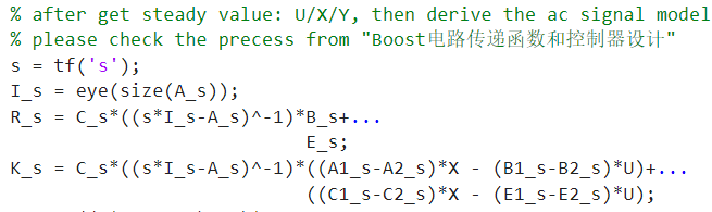
将其进一步的化简为:
y^(s)=︸C[(sI−A)−1 B+E]Ru^(s)+︸{C(sI−A)−1 [(A1−A2)X−(B1−B2)U]+[(C1−C2)X−(E1−E2)U]}Kd^(s)\widehat{\mathbf{y}}\left( \mathbf{s} \right)\mathbf{=}\underset{\mathbf{R}}{\overset{\mathbf{C}\left\lbrack \left( \mathbf{s}\mathbf{I} - \mathbf{A} \right)^{\mathbf{- 1}}\mathbf{\ B}\mathbf{+}\mathbf{E} \right\rbrack}{︸}}\widehat{\mathbf{u}}\left( \mathbf{s} \right)\mathbf{+}\underset{\mathbf{K}}{\overset{\left\{ \mathbf{C}\left( \mathbf{s}\mathbf{I} - \mathbf{A} \right)^{\mathbf{- 1}}\mathbf{\ }\left\lbrack \left( \mathbf{A}_{\mathbf{1}}\mathbf{-}\mathbf{A}_{\mathbf{2}} \right)\mathbf{X}\mathbf{-}\left( \mathbf{B}_{\mathbf{1}}\mathbf{-}\mathbf{B}_{\mathbf{2}} \right)\mathbf{U} \right\rbrack\mathbf{+}\left\lbrack \left( \mathbf{C}_{\mathbf{1}}\mathbf{-}\mathbf{C}_{\mathbf{2}} \right)\mathbf{X}\mathbf{-}\left( \mathbf{E}_{\mathbf{1}}\mathbf{-}\mathbf{E}_{\mathbf{2}} \right)\mathbf{U} \right\rbrack \right\}}{︸}}\widehat{\mathbf{d}}\left( \mathbf{s} \right)y(s)=R︸C[(sI−A)−1 B+E]u(s)+K︸{C(sI−A)−1 [(A1−A2)X−(B1−B2)U]+[(C1−C2)X−(E1−E2)U]}d(s)
化简得到:
y^(s)=Ru^(s)+Kd^(s)[v^(s)]=[R11(s)R12(s)0][v^g(s)i^load(s)0]+[K11(s)]d^(s){\widehat{\mathbf{y}}\left( \mathbf{s} \right)\mathbf{= R}\widehat{\mathbf{u}}\left( \mathbf{s} \right)\mathbf{+ K}\widehat{\mathbf{d}}\left( \mathbf{s} \right)
}{\left\lbrack \widehat{v}(s) \right\rbrack\mathbf{=}\begin{bmatrix}
\mathbf{R}_{\mathbf{11}}\mathbf{(s)} & \mathbf{R}_{\mathbf{12}}\mathbf{(s)} & \mathbf{0}
\end{bmatrix}\begin{bmatrix}
{\widehat{v}}_{g}\left. (s \right.) \\
{\widehat{i}}_{load}\left. (s \right.) \\
0
\end{bmatrix}\mathbf{+}\begin{bmatrix}
\mathbf{K}_{\mathbf{11}}\mathbf{(s)}
\end{bmatrix}\widehat{\mathbf{d}}\left( \mathbf{s} \right)}y(s)=Ru(s)+Kd(s)[v(s)]=[R11(s)R12(s)0]vg(s)iload(s)0+[K11(s)]d(s)
对应的MATLAB脚本如下
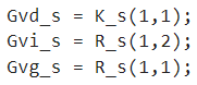
将其展开可得Gvd(s)G_{vd}\left. (s \right.)Gvd(s),Gvi(s)G_{vi}\left. (s \right.)Gvi(s),Gvg(s)G_{vg}\left. (s \right.)Gvg(s)分别是占空比对输出电压的控制传递函数,输出电流对输出电压的扰动传递函数,输入电压对输出电压的扰动传递函数。
Gvd(s)=v^(s)d^(s)∣v^g(s)=0i^load(s)=0=K11(s){G_{vd}\left. (s \right.) = \frac{\widehat{v}(s)}{\widehat{\mathbf{d}}\left( \mathbf{s} \right)}|_{\begin{matrix}
{\widehat{v}}_{g}\left. (s \right.) = 0 \\
{\widehat{i}}_{load}\left. (s \right.) = 0
\end{matrix}} = \mathbf{K}_{\mathbf{11}}\mathbf{(s)}
}Gvd(s)=d(s)v(s)∣vg(s)=0iload(s)=0=K11(s)
Gvi(s)=v^(s)i^load(s)∣v^g(s)=0d^(s)=0=R12(s){G_{vi}\left. (s \right.) = \frac{\widehat{v}(s)}{{\widehat{i}}_{load}\left. (s \right.)}|_{\begin{matrix}
{\widehat{v}}_{g}\left. (s \right.) = 0 \\
\widehat{\mathbf{d}}\left( \mathbf{s} \right) = 0
\end{matrix}} = \mathbf{R}_{\mathbf{12}}\mathbf{(s)}
}Gvi(s)=iload(s)v(s)∣vg(s)=0d(s)=0=R12(s)
Gvg(s)=v^(s)v^g(s)∣i^load(s)=0d^(s)=0=R11(s){G_{vg}\left. (s \right.) = \frac{\widehat{v}(s)}{{\widehat{v}}_{g}\left. (s \right.)}|_{\begin{matrix}
{\widehat{i}}_{load}\left. (s \right.) = 0 \\
\widehat{\mathbf{d}}\left( \mathbf{s} \right) = 0
\end{matrix}} = \mathbf{R}_{\mathbf{11}}\mathbf{(s)}}Gvg(s)=vg(s)v(s)∣iload(s)=0d(s)=0=R11(s)
对应的MATLAB脚本为
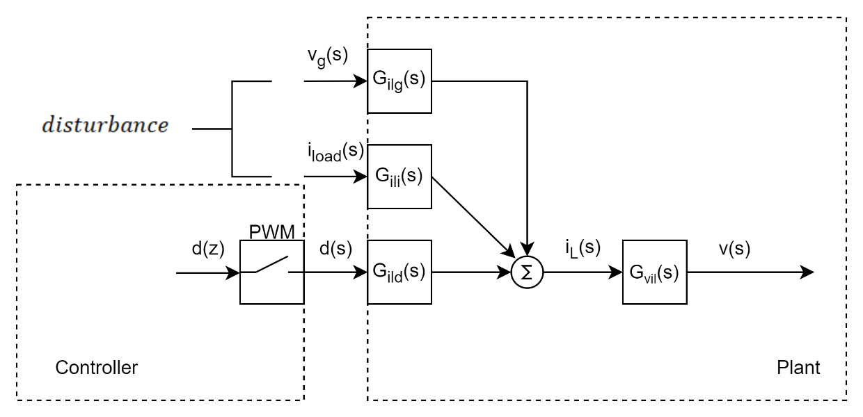
输入电压扰动,输出电流扰动以及占空比扰动组合在一起,输出电压扰动为:
v^(s)=Gvg(s)v^g(s)+Gvi(s)i^load(s)+Gvd(s)d^(s)\widehat{v}(s) = G_{vg}\left. (s \right.){\widehat{v}}_{g}\left. (s \right.) + G_{vi}\left. (s \right.){\widehat{i}}_{load}\left. (s \right.) + G_{vd}\left. (s \right.)\widehat{d}(s)v(s)=Gvg(s)vg(s)+Gvi(s)iload(s)+Gvd(s)d(s)
正如下图所示:

重新化简下式:
x^(t)=︸(sI−A)−1 BM u^(s)+︸(sI−A)−1[(A1−A2)X−(B1−B2)U]Nd^(s)\widehat{x}(t) = \underset{M}{\overset{(sI - A)^{- 1}\ B}{︸}}\ \widehat{u}(s) + \underset{N}{\overset{(sI - A)^{- 1}\left\lbrack \left( A_{1} - A_{2} \right)X - \left( B_{1} - B_{2} \right)U \right\rbrack}{︸}}\widehat{d}(s)x(t)=M︸(sI−A)−1 B u(s)+N︸(sI−A)−1[(A1−A2)X−(B1−B2)U]d(s)
化简得到:
x^(s)=Mu^(s)+Nd^(s)[i^L(s)v^C(s)]=[M11(s)M12(s)0M21(s)M22(s)0][v^g(s)i^load(s)0]+[N11(s)N21(s)]d^(s){\widehat{\mathbf{x}}\left( \mathbf{s} \right)\mathbf{= M}\widehat{\mathbf{u}}\left( \mathbf{s} \right)\mathbf{+ N}\widehat{\mathbf{d}}\left( \mathbf{s} \right)
}{\begin{bmatrix}
{\widehat{i}}_{L}(s) \\
{\widehat{v}}_{C}(s)
\end{bmatrix} = \begin{bmatrix}
M_{11}(s) & M_{12}(s) & 0 \\
M_{21}(s) & M_{22}(s) & 0
\end{bmatrix}\begin{bmatrix}
{\widehat{v}}_{g}\left. (s \right.) \\
{\widehat{i}}_{load}\left. (s \right.) \\
0
\end{bmatrix} + \begin{bmatrix}
N_{11}(s) \\
N_{21}(s)
\end{bmatrix}\widehat{d}(s)}x(s)=Mu(s)+Nd(s)[iL(s)vC(s)]=[M11(s)M21(s)M12(s)M22(s)00]vg(s)iload(s)0+[N11(s)N21(s)]d(s)
MATLAB脚本为:

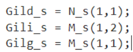
将其展开可得Gild(s)G_{ild}\left. (s \right.)Gild(s),Gili(s)G_{ili}\left. (s \right.)Gili(s),Gilg(s)G_{ilg}\left. (s \right.)Gilg(s)分别是占空比对电感电流的控制传递函数,输出电流对电感电流的扰动传递函数,输入电压对电感电流的扰动传递函数。
Gild(s)=i^L(s)d^(s)∣v^g(s)=0i^load(s)=0=N11(s){G_{ild}\left. (s \right.) = \frac{{\widehat{i}}_{L}(s)}{\widehat{\mathbf{d}}\left( \mathbf{s} \right)}|_{\begin{matrix} {\widehat{v}}_{g}\left. (s \right.) = 0 \\ {\widehat{i}}_{load}\left. (s \right.) = 0 \end{matrix}} = \mathbf{N}_{\mathbf{11}}\mathbf{(s)} }Gild(s)=d(s)iL(s)∣vg(s)=0iload(s)=0=N11(s) Gili(s)=i^L(s)i^load(s)∣v^g(s)=0d^(s)=0=M12(s){G_{ili}\left. (s \right.) = \frac{{\widehat{i}}_{L}(s)}{{\widehat{i}}_{load}\left. (s \right.)}|_{\begin{matrix} {\widehat{v}}_{g}\left. (s \right.) = 0 \\ \widehat{\mathbf{d}}\left( \mathbf{s} \right) = 0 \end{matrix}} = \mathbf{M}_{\mathbf{12}}\mathbf{(s)} }Gili(s)=iload(s)iL(s)∣vg(s)=0d(s)=0=M12(s)Gilg(s)=i^L(s)v^g(s)∣i^load(s)=0d^(s)=0=M11(s){G_{ilg}\left. (s \right.) = \frac{{\widehat{i}}_{L}(s)}{{\widehat{v}}_{g}\left. (s \right.)}|_{\begin{matrix} {\widehat{i}}_{load}\left. (s \right.) = 0 \\ \widehat{\mathbf{d}}\left( \mathbf{s} \right) = 0 \end{matrix}} = \mathbf{M}_{\mathbf{11}}\mathbf{(s)}}Gilg(s)=vg(s)iL(s)∣iload(s)=0d(s)=0=M11(s)
对应的MATLAB脚本为
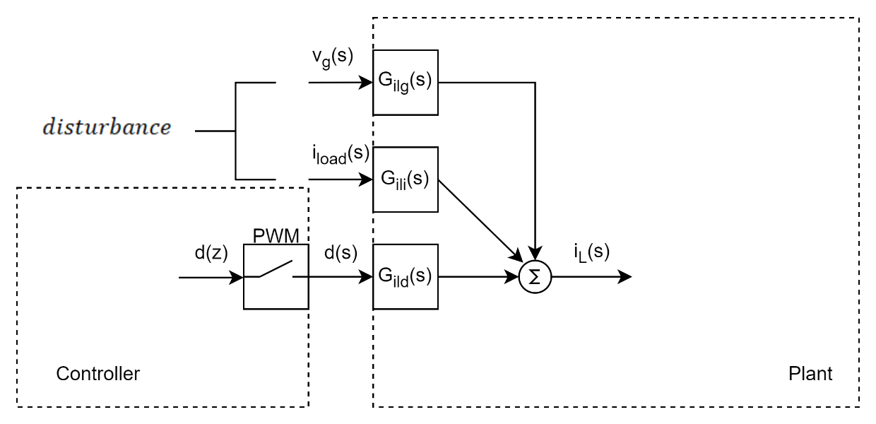
输入电压扰动,输出电流扰动以及占空比扰动组合在一起,电感电流的扰动为:
i^L(s)=Gilg(s)v^g(s)+Gili(s)i^load(s)+Gild(s)d^(s){\widehat{i}}_{L}(s) = G_{ilg}\left. (s \right.){\widehat{v}}_{g}\left. (s \right.) + G_{ili}\left. (s \right.){\widehat{i}}_{load}\left. (s \right.) + G_{ild}\left. (s \right.)\widehat{d}(s)iL(s)=Gilg(s)vg(s)+Gili(s)iload(s)+Gild(s)d(s)
如下图所示
总结,这里得到了影响电感电流和输出电压的控制/扰动传递函数,重新罗列如下:
i^L(s)=︸Gilg(s)v^g(s)+Gili(s)i^load(s)disturbance+︸Gild(s)d^(s)control{\widehat{i}}_{L}(s) = \underset{disturbance}{\overset{G_{ilg}\left. (s \right.){\widehat{v}}_{g}\left. (s \right.) + G_{ili}\left. (s \right.){\widehat{i}}_{load}\left. (s \right.)}{︸}} + \underset{control}{\overset{G_{ild}\left. (s \right.)\widehat{d}(s)}{︸}}iL(s)=disturbance︸Gilg(s)vg(s)+Gili(s)iload(s)+control︸Gild(s)d(s)
v^(s)=︸Gvg(s)v^g(s)+Gvi(s)i^load(s)disturbance+︸Gvd(s)d^(s)control\widehat{v}(s) = \underset{disturbance}{\overset{G_{vg}\left. (s \right.){\widehat{v}}_{g}\left. (s \right.) + G_{vi}\left. (s \right.){\widehat{i}}_{load}\left. (s \right.)}{︸}} + \underset{control}{\overset{G_{vd}\left. (s \right.)\widehat{d}(s)}{︸}}v(s)=disturbance︸Gvg(s)vg(s)+Gvi(s)iload(s)+control︸Gvd(s)d(s)
同时,也可以得到电感电流到输出电压的传递函数,我们可以认为,外部的输入电压和输出电流扰动是先转化为对应的电感电流,然后再转化为对输出电压的影响。
Gvil(s)=v^(s)d^(s)∣v^g(s)=0i^load(s)=0i^L(s)d^(s)∣v^g(s)=0i^load(s)=0=v^(s)i^L(s)G_{vil}\left. (s \right.) = \frac{\frac{\widehat{v}(s)}{\widehat{\mathbf{d}}\left( \mathbf{s} \right)}|_{\begin{matrix} {\widehat{v}}_{g}\left. (s \right.) = 0 \\ {\widehat{i}}_{load}\left. (s \right.) = 0 \end{matrix}}}{\frac{{\widehat{i}}_{L}(s)}{\widehat{\mathbf{d}}\left( \mathbf{s} \right)}|_{\begin{matrix} {\widehat{v}}_{g}\left. (s \right.) = 0 \\ {\widehat{i}}_{load}\left. (s \right.) = 0 \end{matrix}}} = \frac{\widehat{v}(s)}{{\widehat{i}}_{L}(s)}Gvil(s)=d(s)iL(s)∣vg(s)=0iload(s)=0d(s)v(s)∣vg(s)=0iload(s)=0=iL(s)v(s)
如下图所示