沙堆状态的可视化图和雪崩分布

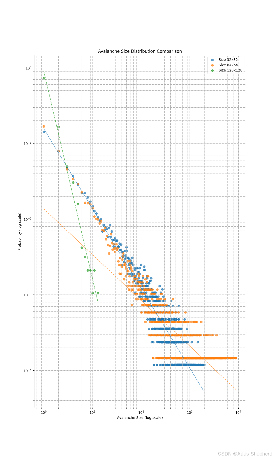
1.自组织临界性​​：

•系统自发演化到临界状态

•雪崩大小分布呈现幂律特征

2.​​尺度不变性​​：

•不同系统尺寸下雪崩分布相似

•幂指数τ与系统尺寸无关

3.​​幂律关系​​：

•双对数坐标下呈现线性关系

•斜率即为幂指数τ

import numpy as np
import matplotlib.pyplot as plt
from matplotlib.colors import ListedColormap
from tqdm import tqdm
from collections import defaultdict
import scipy.stats as statsclass Sandpile:def __init__(self, size=50, critical_value=4):"""初始化沙堆模型参数:size: 网格尺寸 (size x size)critical_value: 临界值，超过此值将发生崩塌"""self.size = sizeself.critical_value = critical_valueself.grid = np.zeros((size, size), dtype=int)self.avalanche_sizes = []  # 存储每次雪崩的大小self.avalanche_durations = []  # 存储每次雪崩的持续时间self.steps = 0def add_sand(self, i=None, j=None):"""在随机位置添加一粒沙子参数:i, j: 指定添加沙子的位置 (如果为None则随机选择)"""if i is None or j is None:i, j = np.random.randint(0, self.size, 2)self.grid[i, j] += 1self.steps += 1return i, jdef topple(self):"""执行崩塌过程，直到网格稳定返回:avalanche_size: 雪崩大小 (崩塌的总次数)duration: 雪崩持续时间 (迭代次数)"""avalanche_size = 0duration = 0topple_queue = []# 找到所有需要崩塌的位置unstable = np.where(self.grid >= self.critical_value)topple_queue = list(zip(unstable[0], unstable[1]))while topple_queue:duration += 1new_topples = []for i, j in topple_queue:# 执行崩塌self.grid[i, j] -= self.critical_valueavalanche_size += 1# 向四个邻居各添加一粒沙子for di, dj in [(0, 1), (1, 0), (0, -1), (-1, 0)]:ni, nj = i + di, j + djif 0 <= ni < self.size and 0 <= nj < self.size:self.grid[ni, nj] += 1# 如果邻居达到临界值，加入下一轮崩塌if self.grid[ni, nj] >= self.critical_value:new_topples.append((ni, nj))# 更新崩塌队列topple_queue = list(set(new_topples))  # 使用set去重return avalanche_size, durationdef simulate(self, n_steps=10000, warmup=1000):"""模拟沙堆演化过程参数:n_steps: 总模拟步数warmup: 预热步数 (达到临界状态前的步数)"""# 预热阶段 (不记录雪崩)for _ in range(warmup):self.add_sand()self.topple()# 主模拟阶段 (记录雪崩)for _ in tqdm(range(n_steps), desc="Simulating sandpile"):self.add_sand()av_size, av_duration = self.topple()if av_size > 0:self.avalanche_sizes.append(av_size)self.avalanche_durations.append(av_duration)def plot_grid(self):"""可视化当前沙堆状态"""cmap = ListedColormap(['white', 'lightblue', 'blue', 'darkblue', 'black'])plt.figure(figsize=(8, 8))plt.imshow(self.grid, cmap=cmap, vmin=0, vmax=self.critical_value)plt.title(f"Sandpile State (Size: {self.size}x{self.size})")plt.colorbar(label='Number of grains')plt.show()def plot_avalanche_distribution(self):"""绘制雪崩大小分布 (双对数坐标)"""if not self.avalanche_sizes:print("No avalanche data available. Run simulation first.")return# 统计雪崩大小频率size_counts = defaultdict(int)for size in self.avalanche_sizes:size_counts[size] += 1sizes = np.array(sorted(size_counts.keys()))freqs = np.array([size_counts[s] for s in sizes])probabilities = freqs / np.sum(freqs)# 过滤掉频率为0的点mask = freqs > 0sizes = sizes[mask]probabilities = probabilities[mask]# 绘制分布图plt.figure(figsize=(10, 6))plt.scatter(sizes, probabilities, alpha=0.7,label=f"Size {self.size}x{self.size}")plt.xscale('log')plt.yscale('log')plt.xlabel('Avalanche Size (log scale)')plt.ylabel('Probability (log scale)')plt.title('Avalanche Size Distribution (Log-Log Plot)')plt.grid(True, which="both", ls="--")# 拟合幂律分布if len(sizes) > 10:slope, intercept, r_value, _, _ = stats.linregress(np.log(sizes), np.log(probabilities))power_law = lambda x: np.exp(intercept) * x ** slopeplt.plot(sizes, power_law(sizes), 'r--',label=f'Power law: τ = {-slope:.2f}\nR² = {r_value ** 2:.2f}')plt.legend()plt.show()# 在不同系统尺寸下运行模拟
sizes = [32, 64, 128]
results = {}for size in sizes:print(f"\nSimulating sandpile of size {size}x{size}")sandpile = Sandpile(size=size)sandpile.simulate(n_steps=20000, warmup=2000)results[size] = sandpile# 绘制沙堆状态sandpile.plot_grid()# 绘制雪崩分布sandpile.plot_avalanche_distribution()# 比较不同系统尺寸的雪崩分布
plt.figure(figsize=(10, 6))
for size, sandpile in results.items():# 统计雪崩大小频率size_counts = defaultdict(int)for av_size in sandpile.avalanche_sizes:size_counts[av_size] += 1sizes_arr = np.array(sorted(size_counts.keys()))freqs = np.array([size_counts[s] for s in sizes_arr])probabilities = freqs / np.sum(freqs)# 过滤掉频率为0的点mask = freqs > 0sizes_arr = sizes_arr[mask]probabilities = probabilities[mask]plt.scatter(sizes_arr, probabilities, alpha=0.7,label=f"Size {size}x{size}")# 添加幂律拟合线if len(sizes_arr) > 10:slope, intercept, _, _, _ = stats.linregress(np.log(sizes_arr), np.log(probabilities))power_law = lambda x: np.exp(intercept) * x ** slopeplt.plot(sizes_arr, power_law(sizes_arr), '--', alpha=0.7)plt.xscale('log')
plt.yscale('log')
plt.xlabel('Avalanche Size (log scale)')
plt.ylabel('Probability (log scale)')
plt.title('Avalanche Size Distribution Comparison')
plt.grid(True, which="both", ls="--")
plt.legend()
plt.show()