当前位置：首页 > news >正文

从头开始学习AI：第四章 - 逻辑回归与分类问题

news 2025/9/6 10:44:01

回顾与引言

在前三章中，我们学习了线性回归用于解决连续值预测问题。然而，机器学习中的许多问题属于分类问题（如垃圾邮件检测、图像分类等）。本章我们将学习逻辑回归——虽然名字中有"回归"，但它实际上是解决二分类问题的经典算法。

逻辑回归的基本概念

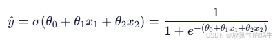
逻辑回归通过sigmoid函数将线性回归的输出映射到(0,1)区间，表示概率：

$h_\theta(x) = \sigma(\theta^Tx) = \frac{1}{1 + e^{-\theta^Tx}}$

其中sigmoid函数为：

$\sigma(z) = \frac{1}{1 + e^{-z}}$

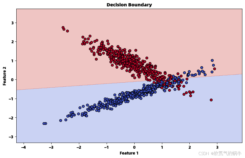
决策边界

当 h_θ(x) ≥ 0.5 时，预测为类别1；当 h_θ(x) < 0.5 时，预测为类别0：

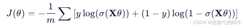
$\hat{y} = \begin{cases} 1 & \text{if } h_\theta(x) \geq 0.5 \\ 0 & \text{if } h_\theta(x) < 0.5 \end{cases}$

成本函数

由于均方误差不适合分类问题，我们使用交叉熵损失函数：

$J(\theta) = -\frac{1}{m}\sum_{i=1}^{m}\left[y^{(i)}\log(h_\theta(x^{(i)})) + (1-y^{(i)})\log(1-h_\theta(x^{(i)}))\right]$

梯度计算

成本函数对参数的梯度：

$\frac{\partial J}{\partial \theta_j} = \frac{1}{m}\sum_{i=1}^{m}(h_\theta(x^{(i)}) - y^{(i)})x_j^{(i)}$

代码实现

import numpy as np
import matplotlib.pyplot as plt
from sklearn.datasets import make_classification
from sklearn.model_selection import train_test_split
from sklearn.preprocessing import StandardScaler
from sklearn.linear_model import LogisticRegression as SklearnLogisticRegression
from sklearn.metrics import accuracy_score, confusion_matrix, classification_reportclass LogisticRegression:"""手动实现逻辑回归算法"""def __init__(self, learning_rate=0.01, n_iterations=1000):"""初始化逻辑回归模型参数:learning_rate -- 学习率 αn_iterations -- 迭代次数"""self.learning_rate = learning_rateself.n_iterations = n_iterationsself.theta = None  # 参数向量self.cost_history = []  # 成本函数历史def _sigmoid(self, z):"""Sigmoid函数: σ(z) = 1 / (1 + e^{-z})参数:z -- 输入值返回:Sigmoid函数值"""return 1 / (1 + np.exp(-z))def _add_intercept(self, X):"""在特征矩阵前添加一列1，用于截距项参数:X -- 特征矩阵 (m, n)返回:添加截距项后的特征矩阵 (m, n+1)"""intercept = np.ones((X.shape[0], 1))return np.concatenate((intercept, X), axis=1)def _compute_cost(self, X, y):"""计算交叉熵成本函数J(θ) = -1/m * Σ[y⁽ⁱ⁾log(hθ(x⁽ⁱ⁾)) + (1-y⁽ⁱ⁾)log(1-hθ(x⁽ⁱ⁾))]参数:X -- 特征矩阵 (包含截距项)y -- 目标向量返回:成本函数值"""m = len(y)h = self._sigmoid(X.dot(self.theta))cost = (-1 / m) * np.sum(y * np.log(h) + (1 - y) * np.log(1 - h))return costdef fit(self, X, y):"""使用梯度下降训练逻辑回归模型参数:X -- 特征矩阵 (m, n)y -- 目标向量 (m,)"""# 添加截距项X_b = self._add_intercept(X)# 初始化参数self.theta = np.zeros(X_b.shape[1])m = len(y)self.cost_history = []# 梯度下降迭代for iteration in range(self.n_iterations):# 计算预测概率z = X_b.dot(self.theta)h = self._sigmoid(z)# 计算梯度: ∇J(θ) = (1/m) * Xᵀ(h - y)gradient = (1 / m) * X_b.T.dot(h - y)# 更新参数: θ := θ - α * ∇J(θ)self.theta -= self.learning_rate * gradient# 记录成本值cost = self._compute_cost(X_b, y)self.cost_history.append(cost)# 每100次迭代打印进度if iteration % 100 == 0:print(f"Iteration {iteration}: Cost = {cost:.6f}")def predict_proba(self, X):"""预测概率值参数:X -- 特征矩阵返回:预测概率值"""X_b = self._add_intercept(X)return self._sigmoid(X_b.dot(self.theta))def predict(self, X, threshold=0.5):"""预测类别参数:X -- 特征矩阵threshold -- 决策阈值返回:预测类别 (0或1)"""probabilities = self.predict_proba(X)return (probabilities >= threshold).astype(int)def plot_decision_boundary(self, X, y):"""绘制决策边界（仅适用于二维特征）参数:X -- 特征矩阵y -- 目标向量"""if X.shape[1] != 2:print("决策边界可视化仅支持二维特征")return# 创建网格点x_min, x_max = X[:, 0].min() - 1, X[:, 0].max() + 1y_min, y_max = X[:, 1].min() - 1, X[:, 1].max() + 1xx, yy = np.meshgrid(np.arange(x_min, x_max, 0.01),np.arange(y_min, y_max, 0.01))# 预测网格点的类别Z = self.predict(np.c_[xx.ravel(), yy.ravel()])Z = Z.reshape(xx.shape)# 绘制决策边界plt.figure(figsize=(10, 6))plt.contourf(xx, yy, Z, alpha=0.3, cmap=plt.cm.coolwarm)plt.scatter(X[:, 0], X[:, 1], c=y, cmap=plt.cm.coolwarm, edgecolors='k')plt.title('Decision Boundary')plt.xlabel('Feature 1')plt.ylabel('Feature 2')plt.show()def plot_cost_history(self):"""绘制成本函数下降曲线"""plt.figure(figsize=(10, 6))plt.plot(self.cost_history)plt.xlabel('Iterations')plt.ylabel('Cost')plt.title('Cost Function History')plt.grid(True)plt.show()def evaluate_model(model, X_test, y_test, model_name="Custom"):"""评估模型性能参数:model -- 训练好的模型X_test -- 测试特征y_test -- 测试标签model_name -- 模型名称"""# 预测y_pred = model.predict(X_test)# 计算准确率accuracy = accuracy_score(y_test, y_pred)print(f"\n=== {model_name} 模型评估 ===")print(f"准确率: {accuracy:.4f}")print("\n混淆矩阵:")print(confusion_matrix(y_test, y_pred))print("\n分类报告:")print(classification_report(y_test, y_pred))return accuracy# 示例使用
if __name__ == "__main__":# 生成二分类数据np.random.seed(42)X, y = make_classification(n_samples=1000, n_features=2, n_redundant=0,n_informative=2, n_clusters_per_class=1,random_state=42)# 数据预处理scaler = StandardScaler()X_scaled = scaler.fit_transform(X)# 划分训练集和测试集X_train, X_test, y_train, y_test = train_test_split(X_scaled, y, test_size=0.2, random_state=42)print("数据形状:")print(f"训练集: {X_train.shape}, 测试集: {X_test.shape}")# 训练自定义逻辑回归模型print("\n=== 训练自定义逻辑回归模型 ===")custom_model = LogisticRegression(learning_rate=0.1, n_iterations=1000)custom_model.fit(X_train, y_train)# 训练scikit-learn逻辑回归模型print("\n=== 训练scikit-learn逻辑回归模型 ===")sklearn_model = SklearnLogisticRegression()sklearn_model.fit(X_train, y_train)# 评估模型custom_accuracy = evaluate_model(custom_model, X_test, y_test, "Custom")sklearn_accuracy = evaluate_model(sklearn_model, X_test, y_test, "Scikit-learn")# 比较结果print(f"\n=== 模型比较 ===")print(f"自定义模型准确率: {custom_accuracy:.4f}")print(f"Scikit-learn准确率: {sklearn_accuracy:.4f}")print(f"准确率差异: {abs(custom_accuracy - sklearn_accuracy):.4f}")# 可视化custom_model.plot_cost_history()custom_model.plot_decision_boundary(X_train, y_train)# 查看模型参数print(f"\n自定义模型参数: {custom_model.theta}")print(f"Scikit-learn参数: 截距={sklearn_model.intercept_}, 系数={sklearn_model.coef_}")

数据形状:
训练集: (800, 2), 测试集: (200, 2)
=== 训练自定义逻辑回归模型 ===
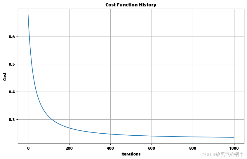
Iteration 0: Cost = 0.677639
Iteration 100: Cost = 0.310346
Iteration 200: Cost = 0.268954
Iteration 300: Cost = 0.254090
Iteration 400: Cost = 0.246750
Iteration 500: Cost = 0.242516
Iteration 600: Cost = 0.239836
Iteration 700: Cost = 0.238029
Iteration 800: Cost = 0.236755
Iteration 900: Cost = 0.235826
=== 训练scikit-learn逻辑回归模型 ===
=== Custom 模型评估 ===
准确率: 0.9000
混淆矩阵:
[[97 7]
[13 83]]
分类报告:
precision recall f1-score support
0 0.88 0.93 0.91 104
1 0.92 0.86 0.89 96
accuracy 0.90 200
macro avg 0.90 0.90 0.90 200
weighted avg 0.90 0.90 0.90 200

=== Scikit-learn 模型评估 ===
准确率: 0.9000
混淆矩阵:
[[97 7]
[13 83]]
分类报告:
precision recall f1-score support
0 0.88 0.93 0.91 104
1 0.92 0.86 0.89 96
accuracy 0.90 200
macro avg 0.90 0.90 0.90 200
weighted avg 0.90 0.90 0.90 200

=== 模型比较 ===
自定义模型准确率: 0.9000
Scikit-learn准确率: 0.9000
准确率差异: 0.0000

自定义模型参数: [ 0.43255724 -0.38866078 3.79220126]
Scikit-learn参数: 截距=[0.6106441], 系数=[[-0.53315119 3.99687498]]

数学原理详解

1. Sigmoid函数及其导数

Sigmoid函数：

$\sigma(z) = \frac{1}{1 + e^{-z}}$

Sigmoid函数的导数：

$\sigma'(z) = \sigma(z)(1 - \sigma(z))$

2. 交叉熵损失函数推导

对于单个样本：

$L(\theta) = -\left[y\log(h_\theta(x)) + (1-y)\log(1-h_\theta(x))\right]$

3. 梯度推导

对参数 θ_j 求偏导：

$\frac{\partial L}{\partial \theta_j} = (h_\theta(x) - y)x_j$

多分类扩展

逻辑回归可以通过以下方式扩展到多分类问题：

1. One-vs-Rest (OvR)

为每个类别训练一个二分类器

2. Softmax回归

$P(y=i|x) = \frac{e^{\theta_i^Tx}}{\sum_{j=1}^{k}e^{\theta_j^Tx}}$

学习心得

通过实现逻辑回归，我理解了：

分类与回归的区别：分类预测离散类别，回归预测连续值
Sigmoid函数的作用：将线性输出映射到概率空间
交叉熵损失的优势：更适合衡量概率分布的差异
决策边界的概念：模型在特征空间中的分类界限

模型评估指标

对于分类问题，常用的评估指标包括：

准确率 (Accuracy)
精确率 (Precision)
召回率 (Recall)
F1分数 (F1-Score)
ROC曲线和AUC

训练流程解析

1：数据放到哪个公式里面训练？

答案：训练数据 (X, y) 被放入“交叉熵损失函数”中，用来计算梯度，从而更新参数。

cost = (-1 / m) * np.sum(y * np.log(h) + (1 - y) * np.log(1 - h))
gradient = (1 / m) * X_b.T.dot(h - y)

数学公式：

这个公式“看到”了所有训练数据
它告诉模型：“你现在预测得不准，要改参数”

2：最后得到的参数又是哪个公式使用的？

答案：最终得到的 theta 被用于“预测公式”中，即 Sigmoid 函数的输入。

z = X_b.dot(self.theta)
h = self._sigmoid(z)

数学公式：

这个公式就是模型本身
theta 是训练过程中学到的“知识”

3：测试样本又是代入到哪个公式？

答案：测试样本代入“预测公式”，先加截距项，再过 Sigmoid，最后根据阈值判断类别。

# 内部执行：
X_b = [[1, x1, x2]]              # 加截距
z = X_b @ theta                  # 线性组合
p = sigmoid(z)                   # 转为概率
y_pred = 1 if p >= 0.5 else 0    # 判决

流程图：

测试样本 [x1, x2]↓
添加截距 → [1, x1, x2]↓
代入线性公式：z = θ₀*1 + θ₁*x1 + θ₂*x2↓
代入 Sigmoid：p = σ(z)↓
判断：p ≥ 0.5 ? → 是→1，否→0↓
输出预测类别

总结图解

训练阶段：
[训练数据 X, y] ↓
放入 交叉熵损失函数 J(θ)↓
计算梯度 ∇J(θ)↓
更新 参数 θ↓
直到损失最小 → 得到最优 θ↘→ [预测公式: P(y=1|x) = σ(θ₀ + θ₁x₁ + θ₂x₂)]↗
预测阶段：
[新样本 x₁, x₂] → 代入预测公式 → 输出概率 → 判决 → 输出类别