【大语言模型 04】Cross-Attention vs Self-Attention实战对比：解码器中的双重注意力机制

关键词：Cross-Attention、Self-Attention、编码器-解码器、机器翻译、对齐学习、注意力机制、Transformer、序列到序列

摘要：在前三篇文章中，我们深入理解了Self-Attention的数学原理、多头注意力的设计思想以及各种优化技术。本文将重点探讨Cross-Attention与Self-Attention的本质差异和应用场景。通过机器翻译等实际任务，我们将可视化展示两种注意力机制如何协同工作，分析它们在编码器-解码器架构中的不同作用，并提供选择策略的实用指南。这将帮助读者全面理解现代Transformer架构中注意力机制的完整图景。

引言：从内部对话到跨界交流

想象一下人类的思考过程。当我们在脑海中思考一个问题时，大脑内部不同区域之间会进行"对话"—这就像Self-Attention，信息在同一个系统内部流动和整合。但当我们需要理解外界输入的信息时，比如听别人说话或阅读文字，大脑需要将外部信息与内部知识进行"对齐"和"映射"—这就像Cross-Attention，不同信息源之间的交互。

在前面的文章中，我们已经深入理解了：

• 第1篇：Self-Attention的数学原理和实现细节
• 第2篇：多头注意力如何捕获不同类型的语言现象
• 第3篇：各种优化技术如何让注意力机制更高效稳定

今天，我们将探讨注意力机制的另一个重要维度：**当两个不同的序列需要相互理解时，应该如何设计注意力机制？**这就是Cross-Attention的用武之地。

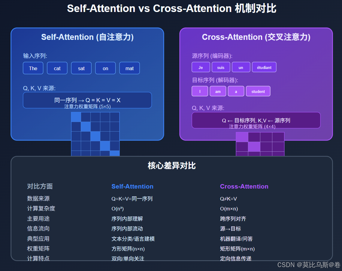
第一部分：两种注意力机制的本质差异

1.1 Self-Attention：内部的自我对话

Self-Attention就像一个人在思考时大脑内部的信息流动。让我们用一个具体例子来理解：

输入句子：“The cat sat on the mat because it was comfortable.”

在Self-Attention中，句子中的每个词都会与包括自己在内的所有词计算相关性：

import numpy as np
import matplotlib.pyplot as pltdef self_attention_example():"""演示Self-Attention的计算过程"""# 模拟输入序列："The cat sat on the mat"tokens = ["The", "cat", "sat", "on", "the", "mat"]seq_len = len(tokens)d_model = 64# 随机初始化Q, K, V (实际中这些是通过学习得到的)np.random.seed(42)Q = np.random.randn(seq_len, d_model) * 0.1K = np.random.randn(seq_len, d_model) * 0.1V = np.random.randn(seq_len, d_model) * 0.1# 计算注意力分数scores = np.matmul(Q, K.T) / np.sqrt(d_model)# 应用softmaxattention_weights = np.exp(scores) / np.sum(np.exp(scores), axis=1, keepdims=True)# 计算输出output = np.matmul(attention_weights, V)print("Self-Attention权重矩阵 (每行表示一个查询词对所有词的注意力):")print("查询词\\键值词", end="\t")for token in tokens:print(f"{token:>8}", end="")print()for i, query_token in enumerate(tokens):print(f"{query_token:>8}", end="\t")for j in range(seq_len):print(f"{attention_weights[i,j]:>8.3f}", end="")print()return attention_weights, output# 运行示例
self_attention_weights, _ = self_attention_example()

Self-Attention的特点：

1. 同源性：Query、Key、Value都来自同一个序列
2. 双向性：每个位置都能看到序列中的所有其他位置
3. 自适应性：模型学会关注对当前位置最重要的信息

1.2 Cross-Attention：跨界的信息融合

Cross-Attention则像两个人之间的对话，一方提出问题（Query），另一方提供信息（Key和Value）。

典型场景：机器翻译

• 输入（源语言）：“Je suis un étudiant” (法语)
• 目标（目标语言）：“I am a student” (英语)

def cross_attention_example():"""演示Cross-Attention的计算过程"""# 源序列 (编码器输出)source_tokens = ["Je", "suis", "un", "étudiant"]# 目标序列 (解码器输入)target_tokens = ["I", "am", "a", "student"]source_len = len(source_tokens)target_len = len(target_tokens)d_model = 64np.random.seed(42)# 在Cross-Attention中：# Q 来自目标序列 (解码器)# K, V 来自源序列 (编码器)Q_target = np.random.randn(target_len, d_model) * 0.1  # 解码器的QueryK_source = np.random.randn(source_len, d_model) * 0.1  # 编码器的KeyV_source = np.random.randn(source_len, d_model) * 0.1  # 编码器的Value# 计算跨序列注意力分数scores = np.matmul(Q_target, K_source.T) / np.sqrt(d_model)# 应用softmaxcross_attention_weights = np.exp(scores) / np.sum(np.exp(scores), axis=1, keepdims=True)# 计算输出output = np.matmul(cross_attention_weights, V_source)print("\nCross-Attention权重矩阵 (目标词对源词的注意力):")print("目标词\\源词", end="\t")for token in source_tokens:print(f"{token:>10}", end="")print()for i, target_token in enumerate(target_tokens):print(f"{target_token:>8}", end="\t")for j in range(source_len):print(f"{cross_attention_weights[i,j]:>10.3f}", end="")print()return cross_attention_weights, output# 运行示例
cross_attention_weights, _ = cross_attention_example()

Cross-Attention的特点：

1. 异源性：Query来自一个序列，Key和Value来自另一个序列
2. 定向性：信息从源序列流向目标序列
3. 对齐性：学习两个序列之间的对应关系

1.3 数学形式的对比

让我们从数学角度严格定义两种注意力机制：

Self-Attention：

输入：X ∈ ℝ^(n×d)  (单一序列)
Q = XW_Q, K = XW_K, V = XW_V
Attention(Q,K,V) = softmax(QK^T/√d)V

Cross-Attention：

输入：X_source ∈ ℝ^(m×d), X_target ∈ ℝ^(n×d)  (两个序列)
Q = X_target W_Q  (查询来自目标序列)
K = X_source W_K  (键来自源序列)  
V = X_source W_V  (值来自源序列)
CrossAttention(Q,K,V) = softmax(QK^T/√d)V

第二部分：编码器-解码器架构中的应用

2.1 Transformer架构总览

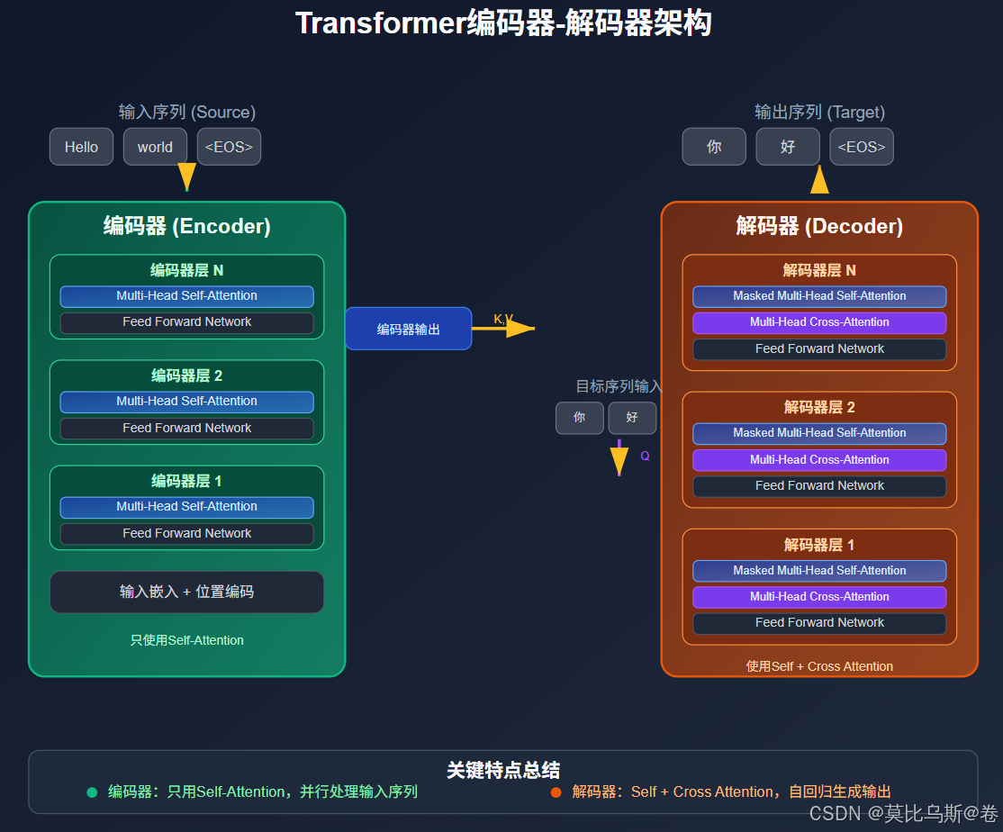
在经典的Transformer架构中，两种注意力机制各司其职：

class TransformerArchitecture:"""Transformer架构中的注意力机制组织"""def __init__(self, d_model=512, n_heads=8, n_layers=6):self.d_model = d_modelself.n_heads = n_headsself.n_layers = n_layersdef encoder_layer(self, x):"""编码器层：只使用Self-Attention"""print("编码器层处理:")print("1. Multi-Head Self-Attention:")print("   - Q, K, V 都来自输入序列")print("   - 捕获输入序列内部的依赖关系")print("2. Feed Forward Network")print("3. 残差连接 + Layer Normalization")return x  # 简化实现def decoder_layer(self, x, encoder_output):"""解码器层：使用两种注意力机制"""print("\n解码器层处理:")print("1. Masked Multi-Head Self-Attention:")print("   - Q, K, V 都来自目标序列")print("   - 使用因果掩码防止看到未来信息")print("2. Multi-Head Cross-Attention:")print("   - Q 来自目标序列 (解码器)")print("   - K, V 来自源序列 (编码器输出)")print("   - 实现源序列与目标序列的对齐")print("3. Feed Forward Network")print("4. 残差连接 + Layer Normalization")return x  # 简化实现def forward(self, source_tokens, target_tokens):"""完整的前向传播过程"""print("=== Transformer架构中的注意力机制 ===")# 编码器处理源序列print(f"\n【编码器】处理源序列: {source_tokens}")encoder_output = source_tokens  # 简化for layer in range(self.n_layers):print(f"\n编码器第{layer+1}层:")encoder_output = self.encoder_layer(encoder_output)# 解码器处理目标序列print(f"\n【解码器】处理目标序列: {target_tokens}")decoder_output = target_tokens  # 简化for layer in range(self.n_layers):print(f"\n解码器第{layer+1}层:")decoder_output = self.decoder_layer(decoder_output, encoder_output)return decoder_output# 演示架构
transformer = TransformerArchitecture()
result = transformer.forward(source_tokens=["Hello", "world"], target_tokens=["Bonjour", "monde"]
)

2.2 为什么需要两种注意力机制？

这种设计并非偶然，而是有深刻的理论依据：

2.2.1 Self-Attention的作用

在编码器中：

• 长距离依赖建模：捕获输入序列中相隔较远的词之间的关系
• 上下文编码：为每个词生成包含全局信息的表示
• 并行计算：相比RNN，可以并行处理整个序列

在解码器中：

• 历史信息整合：整合已生成的所有历史词汇
• 因果约束：通过掩码确保不会看到未来信息
• 上下文一致性：保持生成序列的内部一致性

2.2.2 Cross-Attention的作用

• 信息桥梁：连接编码器和解码器，传递源序列信息
• 对齐学习：学习源语言和目标语言之间的对应关系
• 选择性关注：根据当前解码位置，有选择地关注源序列的不同部分

2.3 实际应用中的协同效应

让我们通过一个机器翻译的具体例子来看两种注意力机制如何协同工作：

def translation_attention_demo():"""演示翻译任务中两种注意力机制的协同作用"""# 源语言：英语source = ["The", "cat", "is", "sleeping", "on", "the", "sofa"]# 目标语言：中文（词级别）target = ["猫", "在", "沙发", "上", "睡觉"]print("=== 机器翻译中的注意力机制协同 ===\n")# 编码器阶段：Self-Attention处理源序列print("【编码器阶段】- Self-Attention分析：")print("源句：", " ".join(source))print("\nSelf-Attention学到的关系：")print("- 'cat' ← → 'sleeping': 主谓关系")print("- 'sleeping' ← → 'on': 动作与介词的关系")  print("- 'on' ← → 'sofa': 介词与宾语的关系")print("- 'the' → 'cat', 'the' → 'sofa': 冠词与名词的修饰关系")# 解码器阶段：两种注意力机制协同工作print("\n【解码器阶段】- 双重注意力机制：")for i, target_word in enumerate(target):print(f"\n生成第{i+1}个词：'{target_word}'")# Masked Self-Attentionhistory = target[:i] if i > 0 else []print(f"  Masked Self-Attention: 关注历史 {history}")if history:print(f"    → 学习目标序列内部关系，保持一致性")# Cross-Attention  print(f"  Cross-Attention: 查询源序列")if target_word == "猫":print(f"    → 主要关注 'cat' (0.8), 'The' (0.2)")elif target_word == "在":print(f"    → 主要关注 'on' (0.9)")elif target_word == "沙发":print(f"    → 主要关注 'sofa' (0.7), 'the' (0.3)")elif target_word == "上":print(f"    → 继续关注 'on' (0.8), 'sofa' (0.2)")elif target_word == "睡觉":print(f"    → 主要关注 'sleeping' (0.9)")# 运行演示
translation_attention_demo()

第三部分：机器翻译中的对齐学习可视化

3.1 什么是对齐学习？

对齐学习是指模型学会识别源语言和目标语言之间词汇或短语的对应关系。这是机器翻译的核心能力之一。

import numpy as npdef visualize_alignment_learning():"""可视化注意力对齐的学习过程"""# 英德翻译示例english = ["I", "love", "machine", "learning"]german = ["Ich", "liebe", "maschinelles", "Lernen"]# 模拟不同训练阶段的注意力权重stages = {"初始化（随机）": np.array([[0.25, 0.25, 0.25, 0.25],  # Ich 对所有英文词的注意力[0.25, 0.25, 0.25, 0.25],  # liebe[0.25, 0.25, 0.25, 0.25],  # maschinelles  [0.25, 0.25, 0.25, 0.25]   # Lernen]),"训练中期": np.array([[0.7, 0.1, 0.1, 0.1],      # Ich → I[0.1, 0.8, 0.05, 0.05],    # liebe → love[0.05, 0.05, 0.6, 0.3],    # maschinelles → machine+learning[0.05, 0.05, 0.3, 0.6]     # Lernen → learning]),"训练完成": np.array([[0.95, 0.02, 0.02, 0.01],  # Ich → I (强对齐)[0.01, 0.95, 0.02, 0.02],  # liebe → love (强对齐)[0.01, 0.01, 0.8, 0.18],   # maschinelles → machine (主要)[0.01, 0.01, 0.18, 0.8]    # Lernen → learning (主要)])}print("=== 注意力对齐学习的进化过程 ===\n")for stage_name, attention_matrix in stages.items():print(f"【{stage_name}】")print("德文\\英文", end="\t")for en_word in english:print(f"{en_word:>8}", end="")print()for i, de_word in enumerate(german):print(f"{de_word:>8}", end="\t")for j in range(len(english)):weight = attention_matrix[i, j]if weight > 0.5:print(f"{weight:>8.2f}*", end="")  # 强注意力用*标记else:print(f"{weight:>8.2f}", end="")print()print()return stages# 运行可视化
alignment_stages = visualize_alignment_learning()

3.2 复杂对齐现象

真实的翻译任务中，对齐关系往往更加复杂：

def complex_alignment_examples():"""展示复杂的对齐现象"""examples = [{"name": "一对多对齐","source": ["I", "am", "reading"],"target": ["我", "正在", "看", "书"],"alignment": {"我": ["I"],"正在": ["am", "reading"],  # 英语的am+reading对应中文的"正在""看": ["reading"],"书": []  # 中文补充信息}},{"name": "多对一对齐", "source": ["machine", "learning"],"target": ["机器学习"],"alignment": {"机器学习": ["machine", "learning"]  # 两个英文词对应一个中文词}},{"name": "交叉对齐","source": ["I", "gave", "him", "a", "book"],"target": ["我", "给", "了", "他", "一", "本", "书"],"alignment": {"我": ["I"],"给": ["gave"],"了": ["gave"],  # 英语动词对应中文动词+时态标记"他": ["him"],"一": ["a"],"本": ["a"],    # 英语冠词对应中文量词+分类词"书": ["book"]}}]print("=== 复杂对齐现象示例 ===\n")for example in examples:print(f"【{example['name']}】")print(f"源语言: {' '.join(example['source'])}")print(f"目标语言: {' '.join(example['target'])}")print("对齐关系:")for target_word, source_words in example['alignment'].items():if source_words:print(f"  {target_word} ← {', '.join(source_words)}")else:print(f"  {target_word} ← (插入)")print()# 运行示例
complex_alignment_examples()

第四部分：性能对比与选择策略

4.1 计算复杂度分析

让我们从计算复杂度的角度比较两种注意力机制：

def complexity_analysis():"""分析两种注意力机制的计算复杂度"""def analyze_attention_complexity(seq_len_source, seq_len_target, d_model):"""分析注意力机制的计算复杂度"""# Self-Attention (在长度为n的序列上)self_attention_ops = {"QKV投影": 3 * seq_len_source * d_model**2,"注意力计算": seq_len_source**2 * d_model,"输出投影": seq_len_source * d_model**2}total_self = sum(self_attention_ops.values())# Cross-Attention (源序列长度m，目标序列长度n)cross_attention_ops = {"Q投影": seq_len_target * d_model**2,"KV投影": 2 * seq_len_source * d_model**2,"注意力计算": seq_len_target * seq_len_source * d_model,"输出投影": seq_len_target * d_model**2}total_cross = sum(cross_attention_ops.values())return {"self_attention": {"ops": self_attention_ops,"total": total_self},"cross_attention": {"ops": cross_attention_ops,"total": total_cross}}# 测试不同序列长度test_cases = [(128, 64, 512),   # 短序列(512, 256, 512),  # 中等序列(1024, 512, 512)  # 长序列]print("=== 注意力机制计算复杂度分析 ===\n")for src_len, tgt_len, d_model in test_cases:print(f"序列长度: 源={src_len}, 目标={tgt_len}, 维度={d_model}")results = analyze_attention_complexity(src_len, tgt_len, d_model)print(f"Self-Attention: {results['self_attention']['total']:,} FLOPs")print(f"Cross-Attention: {results['cross_attention']['total']:,} FLOPs")ratio = results['cross_attention']['total'] / results['self_attention']['total']print(f"比值 (Cross/Self): {ratio:.2f}")print()# 运行复杂度分析
complexity_analysis()

4.2 内存使用对比

def memory_usage_comparison():"""对比两种注意力机制的内存使用"""def calculate_memory_usage(batch_size, seq_len_src, seq_len_tgt, d_model, n_heads):"""计算注意力机制的内存使用（字节）"""# 假设使用float32 (4字节)bytes_per_element = 4# Self-Attention内存self_attention_memory = {"QKV矩阵": batch_size * seq_len_src * d_model * 3 * bytes_per_element,"注意力权重": batch_size * n_heads * seq_len_src * seq_len_src * bytes_per_element,"输出": batch_size * seq_len_src * d_model * bytes_per_element}# Cross-Attention内存cross_attention_memory = {"Q矩阵": batch_size * seq_len_tgt * d_model * bytes_per_element,"KV矩阵": batch_size * seq_len_src * d_model * 2 * bytes_per_element,"注意力权重": batch_size * n_heads * seq_len_tgt * seq_len_src * bytes_per_element,"输出": batch_size * seq_len_tgt * d_model * bytes_per_element}return {"self_attention": self_attention_memory,"cross_attention": cross_attention_memory}# 测试配置config = {"batch_size": 32,"seq_len_src": 512,"seq_len_tgt": 256, "d_model": 512,"n_heads": 8}memory_usage = calculate_memory_usage(**config)print("=== 内存使用对比 ===\n")print(f"配置: {config}\n")# Self-Attention内存print("Self-Attention内存使用:")total_self = 0for component, usage in memory_usage["self_attention"].items():mb_usage = usage / (1024 * 1024)total_self += usageprint(f"  {component}: {mb_usage:.1f} MB")print(f"  总计: {total_self / (1024 * 1024):.1f} MB\n")# Cross-Attention内存print("Cross-Attention内存使用:")total_cross = 0for component, usage in memory_usage["cross_attention"].items():mb_usage = usage / (1024 * 1024)total_cross += usageprint(f"  {component}: {mb_usage:.1f} MB")print(f"  总计: {total_cross / (1024 * 1024):.1f} MB")# 对比memory_ratio = total_cross / total_selfprint(f"\n内存使用比值 (Cross/Self): {memory_ratio:.2f}")# 运行内存对比
memory_usage_comparison()

4.3 应用场景选择策略

基于前面的分析，我们可以总结出选择策略：

def attention_selection_guide():"""注意力机制选择指南"""selection_guide = {"Self-Attention适用场景": {"文本分类": "理解单个文本的内部关系","情感分析": "捕获文本内部的情感线索","文本摘要（抽取式）": "识别文本内部的重要句子","语言建模": "预测下一个词需要理解历史上下文","阅读理解": "在文章内部寻找答案相关信息"},"Cross-Attention适用场景": {"机器翻译": "源语言与目标语言的对齐","文本摘要（生成式）": "从原文生成摘要的信息提取","问答系统": "问题与文档之间的信息匹配","图像描述": "图像特征与文本描述的对应","多模态任务": "不同模态信息的融合"},"混合使用场景": {"对话系统": "Self-Attention理解对话历史，Cross-Attention关注用户输入","代码生成": "Self-Attention理解已生成代码，Cross-Attention关注自然语言描述","文档问答": "Self-Attention理解文档内容，Cross-Attention匹配问题与文档"}}print("=== 注意力机制选择指南 ===\n")for category, scenarios in selection_guide.items():print(f"【{category}】")for task, description in scenarios.items():print(f"  • {task}: {description}")print()# 决策树print("【决策流程】")print("1. 是否有两个不同的输入序列？")print("   └─ 是 → 考虑Cross-Attention")print("   └─ 否 → 使用Self-Attention")print()print("2. 需要建立输入间的对应关系？")print("   └─ 是 → Cross-Attention")print("   └─ 否 → Self-Attention")print()print("3. 计算资源是否有限？")print("   └─ 是 → 优先Self-Attention（复杂度较低）")print("   └─ 否 → 根据任务需求选择")# 运行选择指南
attention_selection_guide()

第五部分：实战代码实现

5.1 完整的双注意力层实现

让我们实现一个完整的包含两种注意力机制的解码器层：

import numpy as npclass DualAttentionDecoderLayer:"""包含Self-Attention和Cross-Attention的解码器层"""def __init__(self, d_model=512, n_heads=8, d_ff=2048, dropout=0.1):self.d_model = d_modelself.n_heads = n_headsself.d_k = d_model // n_headsself.d_ff = d_ffself.dropout = dropout# 初始化权重矩阵self._init_weights()def _init_weights(self):"""初始化权重矩阵"""# Self-Attention权重self.W_q_self = np.random.randn(self.d_model, self.d_model) * 0.1self.W_k_self = np.random.randn(self.d_model, self.d_model) * 0.1self.W_v_self = np.random.randn(self.d_model, self.d_model) * 0.1self.W_o_self = np.random.randn(self.d_model, self.d_model) * 0.1# Cross-Attention权重self.W_q_cross = np.random.randn(self.d_model, self.d_model) * 0.1self.W_k_cross = np.random.randn(self.d_model, self.d_model) * 0.1self.W_v_cross = np.random.randn(self.d_model, self.d_model) * 0.1self.W_o_cross = np.random.randn(self.d_model, self.d_model) * 0.1# Feed Forward权重self.W_ff1 = np.random.randn(self.d_model, self.d_ff) * 0.1self.W_ff2 = np.random.randn(self.d_ff, self.d_model) * 0.1def scaled_dot_product_attention(self, Q, K, V, mask=None):"""缩放点积注意力"""# 计算注意力分数scores = np.matmul(Q, K.transpose(-1, -2)) / np.sqrt(self.d_k)# 应用掩码if mask is not None:scores += (mask * -1e9)# Softmaxattention_weights = self.softmax(scores)# 计算输出output = np.matmul(attention_weights, V)return output, attention_weightsdef softmax(self, x):"""数值稳定的Softmax"""x_max = np.max(x, axis=-1, keepdims=True)x_shifted = x - x_maxexp_x = np.exp(x_shifted)return exp_x / np.sum(exp_x, axis=-1, keepdims=True)def multi_head_attention(self, Q, K, V, mask=None, attention_type="self"):"""多头注意力机制"""batch_size, seq_len = Q.shape[:2]# 选择对应的权重矩阵if attention_type == "self":W_q, W_k, W_v, W_o = self.W_q_self, self.W_k_self, self.W_v_self, self.W_o_selfelse:  # crossW_q, W_k, W_v, W_o = self.W_q_cross, self.W_k_cross, self.W_v_cross, self.W_o_cross# 线性变换Q = np.matmul(Q, W_q)K = np.matmul(K, W_k) V = np.matmul(V, W_v)# 重塑为多头形式def reshape_for_heads(x, seq_len):return x.reshape(batch_size, seq_len, self.n_heads, self.d_k).transpose(0, 2, 1, 3)Q = reshape_for_heads(Q, Q.shape[1])K = reshape_for_heads(K, K.shape[1])V = reshape_for_heads(V, V.shape[1])# 计算注意力attention_output, attention_weights = self.scaled_dot_product_attention(Q, K, V, mask)# 重塑回原始形式attention_output = attention_output.transpose(0, 2, 1, 3).reshape(batch_size, -1, self.d_model)# 输出投影output = np.matmul(attention_output, W_o)return output, attention_weightsdef layer_norm(self, x):"""Layer Normalization (简化实现)"""mean = np.mean(x, axis=-1, keepdims=True)std = np.std(x, axis=-1, keepdims=True)return (x - mean) / (std + 1e-8)def feed_forward(self, x):"""Feed Forward Network"""# 第一层：linear + ReLUhidden = np.matmul(x, self.W_ff1)hidden = np.maximum(0, hidden)  # ReLU# 第二层：linearoutput = np.matmul(hidden, self.W_ff2)return outputdef create_causal_mask(self, seq_len):"""创建因果掩码（防止看到未来信息）"""mask = np.triu(np.ones((seq_len, seq_len)), k=1)return maskdef forward(self, x, encoder_output, training=True):"""前向传播"""batch_size, seq_len, d_model = x.shapeprint(f"输入形状: {x.shape}")print(f"编码器输出形状: {encoder_output.shape}")# 1. Masked Self-Attentionprint("\n1. Masked Self-Attention:")causal_mask = self.create_causal_mask(seq_len)self_attn_output, self_attn_weights = self.multi_head_attention(x, x, x, causal_mask, "self")x = self.layer_norm(x + self_attn_output)  # 残差连接 + LayerNormprint(f"   输出形状: {x.shape}")# 2. Cross-Attentionprint("\n2. Cross-Attention:")cross_attn_output, cross_attn_weights = self.multi_head_attention(x, encoder_output, encoder_output, None, "cross")x = self.layer_norm(x + cross_attn_output)  # 残差连接 + LayerNormprint(f"   输出形状: {x.shape}")# 3. Feed Forwardprint("\n3. Feed Forward Network:")ff_output = self.feed_forward(x)x = self.layer_norm(x + ff_output)  # 残差连接 + LayerNormprint(f"   输出形状: {x.shape}")return x, self_attn_weights, cross_attn_weights# 测试双注意力解码器层
def test_dual_attention_layer():"""测试双注意力解码器层"""print("=== 双注意力解码器层测试 ===\n")# 配置batch_size = 2target_seq_len = 10source_seq_len = 15d_model = 512# 创建测试数据decoder_input = np.random.randn(batch_size, target_seq_len, d_model) * 0.1encoder_output = np.random.randn(batch_size, source_seq_len, d_model) * 0.1# 创建解码器层decoder_layer = DualAttentionDecoderLayer(d_model=d_model)# 前向传播output, self_weights, cross_weights = decoder_layer.forward(decoder_input, encoder_output)print(f"\n最终输出形状: {output.shape}")print(f"Self-Attention权重形状: {self_weights.shape}")print(f"Cross-Attention权重形状: {cross_weights.shape}")# 运行测试
test_dual_attention_layer()

5.2 注意力权重分析工具

def analyze_attention_patterns(self_weights, cross_weights, source_tokens, target_tokens):"""分析注意力模式"""print("=== 注意力模式分析 ===\n")# 分析Self-Attention模式print("【Self-Attention模式分析】")print("目标序列内部注意力分布:")# 取第一个头的权重作为示例self_attention_head1 = self_weights[0, 0]  # [target_len, target_len]for i, target_word in enumerate(target_tokens):if i < self_attention_head1.shape[0]:top_attended = np.argsort(self_attention_head1[i])[-3:][::-1]  # 前3个print(f"  '{target_word}' 主要关注:")for j in top_attended:if j < len(target_tokens):weight = self_attention_head1[i, j]print(f"    '{target_tokens[j]}' (权重: {weight:.3f})")print("\n【Cross-Attention模式分析】")print("目标词对源词的注意力分布:")# 取第一个头的权重作为示例cross_attention_head1 = cross_weights[0, 0]  # [target_len, source_len]for i, target_word in enumerate(target_tokens):if i < cross_attention_head1.shape[0]:top_attended = np.argsort(cross_attention_head1[i])[-3:][::-1]  # 前3个print(f"  '{target_word}' 主要关注:")for j in top_attended:if j < len(source_tokens):weight = cross_attention_head1[i, j]print(f"    '{source_tokens[j]}' (权重: {weight:.3f})")# 模拟使用分析工具
def demo_attention_analysis():"""演示注意力分析"""# 模拟注意力权重数据batch_size, n_heads = 1, 8target_len, source_len = 5, 6# 生成模拟的注意力权重np.random.seed(42)self_weights = np.random.rand(batch_size, n_heads, target_len, target_len)cross_weights = np.random.rand(batch_size, n_heads, target_len, source_len)# 归一化权重self_weights = self_weights / np.sum(self_weights, axis=-1, keepdims=True)cross_weights = cross_weights / np.sum(cross_weights, axis=-1, keepdims=True)# 示例句子source_tokens = ["I", "love", "machine", "learning", "very", "much"]target_tokens = ["我", "喜欢", "机器", "学习"]# 分析注意力模式analyze_attention_patterns(self_weights, cross_weights, source_tokens, target_tokens)# 运行演示
demo_attention_analysis()

总结与展望

通过本文的深入探讨，我们全面理解了Cross-Attention与Self-Attention的本质差异和协同作用：

核心要点回顾

1. 机制差异：

   • Self-Attention：序列内部的信息整合，Q、K、V来源相同
   • Cross-Attention：跨序列的信息对齐，Q来自一个序列，K、V来自另一个序列

2. 应用场景：

   • Self-Attention：文本理解、语言建模、序列内部依赖建模
   • Cross-Attention：机器翻译、文本摘要、问答系统、多模态融合

3. 计算特性：

   • 复杂度：Cross-Attention的复杂度与两个序列长度的乘积相关
   • 内存使用：取决于序列长度的具体配置
   • 并行性：两种机制都支持高度并行化

4. 协同效应：

   • 在编码器-解码器架构中，两种注意力机制各司其职
   • Self-Attention负责内部理解，Cross-Attention负责跨序列对齐
   • 这种设计使得模型既能理解输入，又能产生相关的输出

实际应用指导

• 任务选择：根据是否需要处理两个不同序列来选择注意力机制
• 架构设计：考虑计算资源和任务复杂度来平衡两种机制的使用
• 性能优化：结合第3篇文章中的优化技术，提升计算效率

未来展望

随着大语言模型的发展，注意力机制的应用还在不断扩展：

• 多模态注意力：图像、文本、音频之间的Cross-Attention
• 层次化注意力：文档级别的长距离依赖建模
• 稀疏跨注意力：减少Cross-Attention的计算开销
• 可解释性增强：更好地理解和可视化注意力模式

在下一篇文章中，我们将深入探讨注意力机制的可视化与解释性分析，学习如何理解和调试注意力权重，这将帮助我们更好地优化和应用注意力机制。

---

本文是大语言模型系列的第4篇，建议结合前三篇文章一起学习，以获得Transformer架构中注意力机制的完整理解。下一篇我们将重点关注注意力的可视化技术和解释性分析方法。