数据分析专栏记录之 -基础数学与统计知识
数据分析专栏记录之 -基础数学与统计知识:
1、描述性统计
'''均值'''
data_set = [10, 20, 30, 40, 50]
mean = sum(data_set)/len(data_set)'''np  里面的函数,对二维进行操作时,   默认每一列 '''
mean1 = np.mean(data_set)
print(mean, mean1)s = 0
for i in data_set:s = s + i
print(s/len(data_set))
30.0 30.0
30.0
""" 平均数  、  加权平均数  的实现"""
import numpy as np
average = np.average(data_set)
print(average)weight_average = np.average(data_set, weights=[1, 2, 1, 2, 1])
print(weight_average)
30.0
30.0
"""标准差  /  均方差 / 欧氏距离"""
import numpy as np
std = np.std(data_set)
print(std)"""方差"""var = np.var(data_set)
print(var)def avg(var_Calculation):s = 0for i in var_Calculation:s = s+ireturn (s/len(var_Calculation))
av = avg(data_set)
sum_var = 0
for i in data_set:sum_var += ((i-av)**2)
print(sum_var/len(data_set))
14.142135623730951
200.0
200.0
"""中位数"""
print(np.median(data_set))speed = [99,86,87,88,111,86,103,87,94,78,77,85,86]
i = 0
while i<=len(speed)-2:j = i+1while j <= len(speed)-1:if speed[i] < speed[j]:t = speed[i]speed[i] = speed[j]speed[j] = tj = j+1i = i+1if len(speed)%2 ==1:print(speed[int(len(speed)/2)])
else:print((speed[int(len(speed)/2)] + speed[int(len(speed)/2)-1])/2)
30.0
87
"""众数"""
from scipy import stats
speed = [99,86,87,88,111,86,103,87,94,78,77,85,86]
x = stats.mode(speed)
print(x)zd = {}
for i in speed:zd[i]=0
print(zd)for j in speed:if j in zd.keys():zd[j] += 1
print(zd)maxkey = 0
maxvalue = 0
for key in zd.keys():if zd[key]>maxvalue:maxkey = keymaxvalue = zd[key]
print(maxkey, maxvalue)
ModeResult(mode=np.int64(86), count=np.int64(3))
{99: 0, 86: 0, 87: 0, 88: 0, 111: 0, 103: 0, 94: 0, 78: 0, 77: 0, 85: 0}
{99: 1, 86: 3, 87: 2, 88: 1, 111: 1, 103: 1, 94: 1, 78: 1, 77: 1, 85: 1}
86 3
"""
百分位数
例如:假设我们有一个数组,包含住在一条街上的人的年龄。
ages = [5,31,43,48,50,41,7,11,15,39,80,82,32,2,8,6,25,36,27,61,31]
什么是 75 百分位数?答案是 43,这意味着 75% 的人是 43 岁或以下。
"""
ages = [5,31,43,48,50,41,7,11,15,39,80,82,32,2,8,6,25,36,27,61,31]
x = np.percentile(ages, 80)
print(x)def per(sz, pe):sz.sort()slen = len(sz)return sz[int((pe * slen)/100)]
print(per(ages, 80))
48.0
48
"""
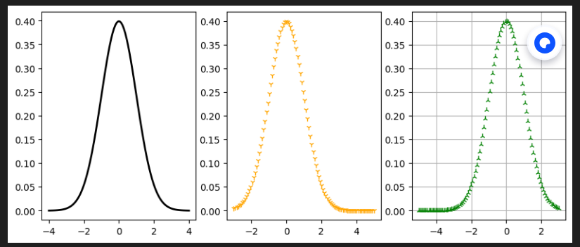
定义:偏度(skewness),是统计数据分布偏斜方向和程度的度量,或者说是统计数据分布非对称程度的数字特征。说人话:偏度或偏态系数或偏度系数(Skewness)用来度量分布是否对称,一个分布如果不对称,则被称为偏度。分布分为三种:对称分布(正态分布)、正偏分布(右偏分布)、负偏分布(左偏分布)
对称分布的特点:左右对称,均值 = 中位数 = 众数,偏度 = 0
正偏分布的特点:右侧长尾,均值 >中位数 >众数,偏度 > 0
负偏分布的特点:左侧长尾,均值 < 中位数 < 众数,偏度 < 0step
绘制图像展示
"""
import numpy as np
import matplotlib.pyplot as plt
from scipy import stats
fig, axs = plt.subplots(1, 3, figsize=(10, 4))def plot():""" 标准正态 :draw standard deviation normal distribution"""mu = 0.0 #均值sd = 1.0 #标准差x = np.linspace(mu-4*sd, mu+4*sd, 100)y = stats.norm.pdf(x)""" 正偏分布 """x1 = np.linspace(mu-3*sd, mu+5*sd, 100)y1 = stats.norm.pdf(x1)""" 负偏分布 """x2 = np.linspace(mu-5*sd, mu+3*sd, 100)y2 = stats.norm.pdf(x2)axs[0].plot(x, y, "g", linewidth=2, color='black')axs[1].plot(x1, y1, "g1", linewidth=2, color='orange')axs[2].plot(x2, y2, "g2", linewidth=2, color='green')plt.grid(True)plt.show()if __name__ == '__main__':plot()
"""
偏度:
根据数据, 计算均值、中位数、众数  得出偏度
"""
import pandas as pd
from scipy import stats
import numpy as np
speed_ = [1,4,6,8,10,20]# 计算公式1
mean = np.mean(speed_)
std = np.std(speed_, ddof=1)
n = len(speed_)
a1 = sum(((speed_-mean)/std)**3)
a2 = a1*(n)/((n-1)*(n-2))
print("偏度:",a2)# 计算公式2
mean = np.mean(speed_)
std = np.std(speed_, ddof=1)
n = len(speed_)
a1 = sum(((speed_-mean)/std)**3)
a2 = a1/(n)
print(a2)'''
可以看到使用不同公式计算得到的偏度不同:
公式1得到的偏度:1.2737636108819756
公式2得到的偏度:0.7076464504899865
'''# 调用函数计算
d = stats.skew(speed_, bias=False)
print("偏度:", d)
偏度: 1.2737636108819756
0.7076464504899865
偏度: 1.2737636108819756
计算公式1:
S=n(n−1)(n−2)∑i=1n[(Xi−μσ)3]S=\frac{n}{(n-1)(n-2)} \sum_{i=1}^{n}\left[\left(\frac{X_{i}-\mu}{\sigma}\right)^{3}\right]S=(n−1)(n−2)n∑i=1n[(σXi−μ)3]
计算公式2:
S=1n∑i=1n[(Xi−μσ)3]S=\frac{1}{n} \sum_{i=1}^{n}\left[\left(\frac{X_{i}-\mu}{\sigma}\right)^{3}\right]S=n1∑i=1n[(σXi−μ)3]
"""
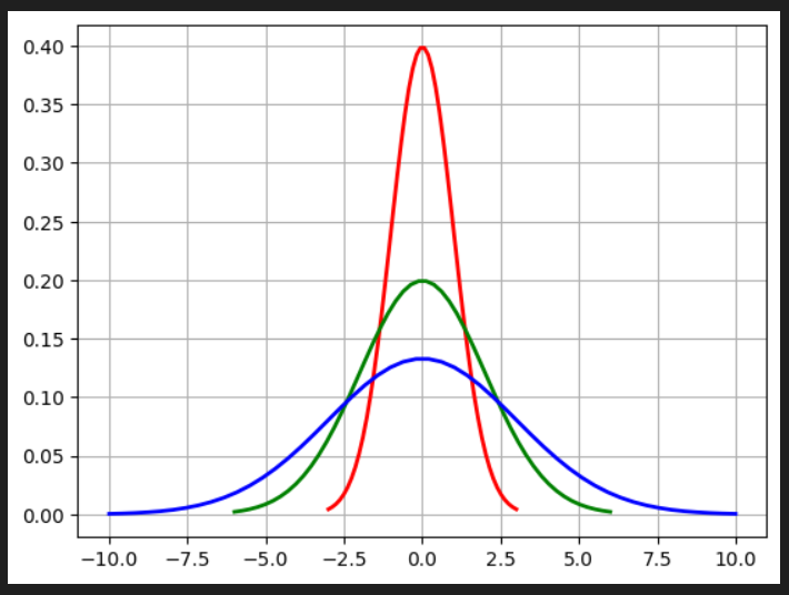
峰度
定义:峰度(peakedness;kurtosis)又称峰态系数。表征概率密度分布曲线在平均值处峰值高低的特征数。
说人话:峰度反映了峰部的尖度,用来度量数据在中心聚集程度,峰度越大分布图越尖,峰度越小分布图越矮胖。
"""import numpy as np
import matplotlib.pyplot as plt
from scipy import statsdef plot():"""draw standard deviation normal distribution"""mu = 0.0 # meansd1 = 1.0 # stdsd2 = 2.0sd3 = 3.0# 特征:x参数一致,但是扩散开的程度不一样。y不一致,向上的程度不一样# red linex = np.linspace(mu-3*sd1, mu+3*sd1, 50)y = stats.norm.pdf(x)plt.plot(x, y , "r", linewidth=2)# green linex2 = np.linspace(mu-6*sd1, mu+6*sd1, 50)y2 = stats.norm.pdf(x2, mu, sd2)plt.plot(x2, y2, "g", linewidth=2)# blue linex3 = np.linspace(mu-10*sd1, mu+10*sd1, 50)y3 = stats.norm.pdf(x3, mu, sd3)plt.plot(x3, y3, "b", linewidth=2)plt.grid(True) # 显示网格线plt.show()if __name__ == '__main__':plot()
"""
对于正态分布来说峰度=3,部分统计软件会给出超额峰度,超额峰度=峰度-3。
中锋分布的超额峰度=0, 尖峰分布的超额峰度>0,低峰分布的超额峰度<0。
"""import numpy as np
import pandas as pd
from scipy import statsarr = np.array([1,4,6,8,10,20])
#标准差
std = stats.tstd(arr, ddof=1)
# 偏度
skew_ = stats.skew(arr, bias=False)
# 峰度
e = stats.kurtosis(arr, bias=False)
print(e)"""  面对pd数据  """
data = pd.DataFrame(arr)
print(data.kurt())
2.154642470375478
0    2.154642
dtype: float64
"""一维数据 曲线图"""
import pandas as pd
import matplotlib.pyplot as plt
import seaborn as sns
import numpy as np# 读取csv文件
reviews = pd.read_csv("/content/drive/MyDrive/数据分析/HC.csv")# 第一列、第二列的数据
# print(reviews['0'], reviews['0.1'])
# 绘制曲线图
plt.plot(reviews['0'], reviews['0.1'])
plt.xlabel('Time')
plt.ylabel("Position")
plt.title("Position vs Time")
plt.tight_layout()
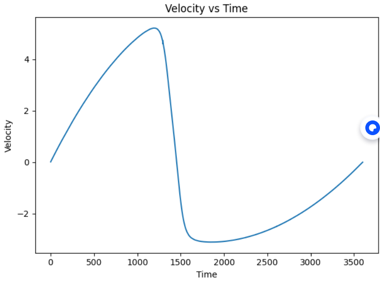
plt.show()# 根据速度 求 加速度, 绘制加速度曲线,【 time a 】
t = reviews['0']
s = reviews['0.1']
# 计算速度 (前向差分法)
velocity = np.diff(s)/ np.diff(t) # v = Δp / Δt
# 为了方便绘图,给速度数组添加一个最后值,与时间点对齐
velocity = np.append(velocity, velocity[-1])
# 绘制位置和速度的图像
plt.plot(reviews['0'], velocity*100)
plt.xlabel('Time')
plt.ylabel("Velocity")
plt.title("Velocity vs Time")
plt.tight_layout()
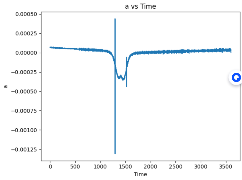
plt.show()# 根据速度 求 加速度, 绘制加速度曲线,【 time a 】
t = reviews['0']
# 计算速度 (前向差分法)
Acceleration = np.diff(velocity)/ np.diff(t) # v = Δp / Δt
# 为了方便绘图,给速度数组添加一个最后值,与时间点对齐
Acceleration = np.append(Acceleration, Acceleration[-1])
# 绘制位置和速度的图像
plt.plot(reviews['0'], Acceleration)
plt.xlabel('Time')
plt.ylabel("a")
plt.title("a vs Time")
plt.tight_layout()
plt.show()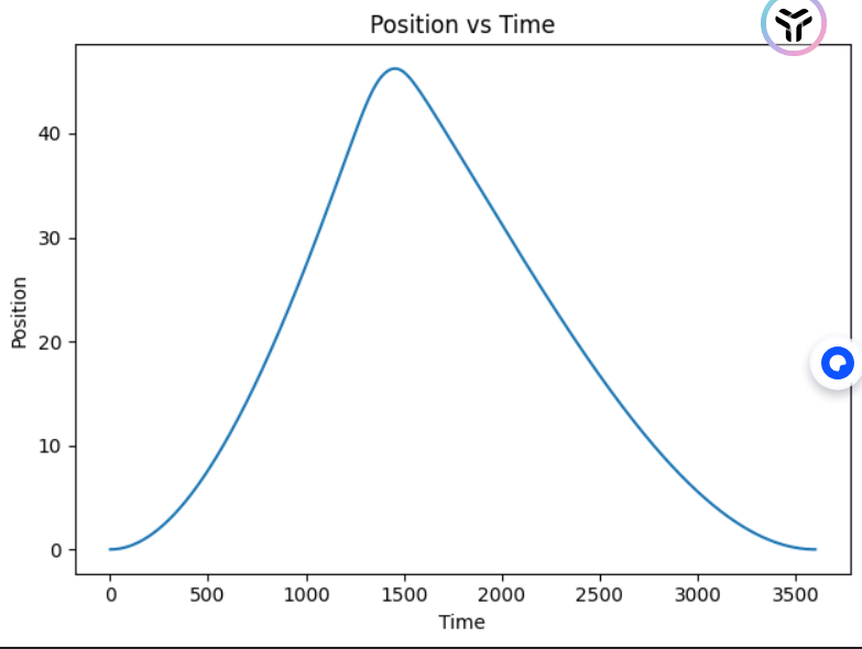
import pandas as pd
import matplotlib.pyplot as plt
import numpy as np# 读取 CSV 文件
reviews = pd.read_csv("/content/drive/MyDrive/数据分析/HC.csv")# 时间 (t) 和位置 (s)
t = reviews['0'].to_numpy()
s = reviews['0.1'].to_numpy()# === 使用中心差分法计算速度和加速度 ===
velocity = np.gradient(s, t)           # 速度 v = ds/dt
acceleration = np.gradient(velocity, t) # 加速度 a = dv/dt# === 绘制三个曲线 ===
plt.figure(figsize=(10, 8))# 路程-时间
plt.subplot(3, 1, 1)
plt.plot(t, s, 'b', linewidth=2)
plt.ylabel('Position')
plt.title('Position, Velocity, and Acceleration vs Time')# 速度-时间
plt.subplot(3, 1, 2)
plt.plot(t, velocity, 'g', linewidth=2)
plt.ylabel('Velocity')# 加速度-时间
plt.subplot(3, 1, 3)
plt.plot(t, acceleration, 'r', linewidth=2)
plt.xlabel('Time')
plt.ylabel('Acceleration')plt.tight_layout()
plt.show()# === 计算指定时间点的速度(例如 t=2.5s)===
target_time = 2.5
velocity_at_target = np.interp(target_time, t, velocity)
print(f"t = {target_time}s 时的速度: {velocity_at_target:.4f}")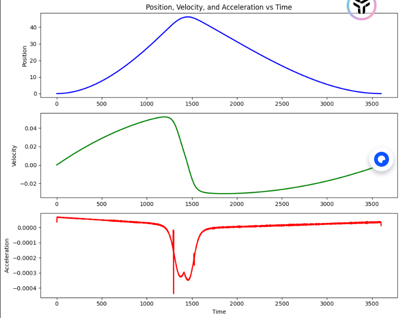
致谢
靠咖啡续命的牛马,👍点赞 📁 关注 💬评论 💰打赏。
参考
[1] deepseek等ai
往期回顾
- 无,新手上车